8. Dispersal limitation
One of the most disputed assumptions of species distribution models is that species are at equilibrium with their environment. This assumptions means that species are supposed to occupy their full range of suitable environmental conditions. In reality, it is unlikely, because of dispersal limitations, biotic interactions, etc., which precludes species to occupy areas which are theoretically suitable. As a consequence, it is worth testing how well modelling techniques perform when this assumption is violated.
This is why we introduced the possibility of biasing the distribution
of species, to simulate species which are not at equilibrium. This
possibility is implemented in the function
limitDistribution.
8.1. An introduction example
Let’s use the same virtual species we generated above:
library(virtualspecies)## Le chargement a nécessité le package : terra## terra 1.7.46## The legacy packages maptools, rgdal, and rgeos, underpinning the sp package,
## which was just loaded, will retire in October 2023.
## Please refer to R-spatial evolution reports for details, especially
## https://r-spatial.org/r/2023/05/15/evolution4.html.
## It may be desirable to make the sf package available;
## package maintainers should consider adding sf to Suggests:.
## The sp package is now running under evolution status 2
## (status 2 uses the sf package in place of rgdal)library(geodata)
# Worldclim data
worldclim <- worldclim_global(var = "bio", res = 10,
path = tempdir())
names(worldclim) <- paste0("bio", 1:19)
# Formatting of the response functions
my.parameters <- formatFunctions(bio1 = c(fun = 'dnorm', mean = 25, sd = 5),
bio12 = c(fun = 'dnorm', mean = 4000, sd = 2000))
# Generation of the virtual species
my.first.species <- generateSpFromFun(raster.stack = worldclim[[c("bio1", "bio12")]],
parameters = my.parameters)## Generating virtual species environmental suitability...## - The response to each variable was rescaled between 0 and 1. To
## disable, set argument rescale.each.response = FALSE## - The final environmental suitability was rescaled between 0 and 1. To disable, set argument rescale = FALSE# Conversion to presence-absence
my.first.species <- convertToPA(my.first.species,
beta = 0.7, plot = FALSE)## --- Determing species.prevalence automatically according to alpha and beta## Logistic conversion finished:
##
## - beta = 0.7
## - alpha = -0.05
## - species prevalence =0.0246147220541227Now, let’s assume our species originates from South America, and has not been able to disperse through the oceans (result in figure 8.2).
my.first.species <- limitDistribution(my.first.species,
                                      geographical.limit = "continent",
                                      area = "South America",
                                      plot = FALSE)

par(mfrow = c(2, 1))
plot(my.first.species$pa.raster, main = "Theoretical distribution")
plot(my.first.species$occupied.area, main = "Realised distribution")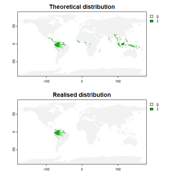
In the following sections, we see how to customise this function, but the usage is basically the same as when applying a sampling bias.
8.2. Customisation of the parameters
There are six main possibilities to limit the distribution to a particular area.
8.2.1. Using countries, regions or continents
As illustrated in the example above, use
geographical.limit = "country",
geographical.limit = continent or
geographical.limit = "region" and provide the correct
name(s) of the area to area
my.sp1 <- limitDistribution(my.first.species,
                            geographical.limit = "country",
                            area = c("Brazil", "Venezuela"))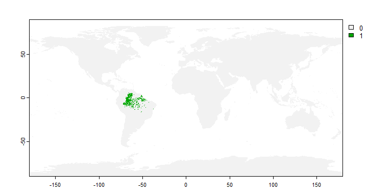
8.2.2. Using a polygon
Set geographical.limit = "polygon", and provide a
polygon (of type SpatVector from terra or
sf from package sf) to the argument
area.
philippines <- rnaturalearth::ne_countries(country = "Philippines",
                                           returnclass = "sf")
my.sp2 <- limitDistribution(my.first.species,
                            geographical.limit = "polygon",
                            area = philippines)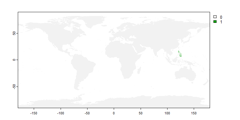
8.2.3. Using an extent object
Set geographical.limit = "extent", and provide an extent
to the argument area (see section
7.2.3. if you are not familiar with extents). You can also draw
manually a polygon or extent on the map by simply setting
geographical.limit = "polygon" or
geographical.limit = "extent", and clicking on the map when
asked to:
my.extent <- ext(-80, -20, -35, -5)
my.sp2 <- limitDistribution(my.first.species,
                            geographical.limit = "extent",
                            area = my.extent)
plot(my.extent, add = TRUE)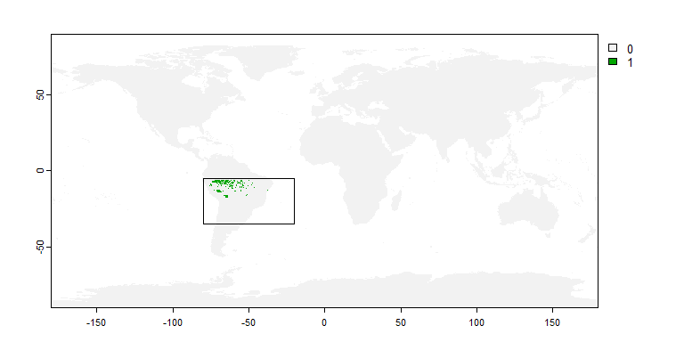
8.2.4. Using a raster of suitable habitat
Let’s first generate an example raster of habitat patches. For this, I will use a function to generate artificial habitat patches that you can find here..
suitable.habitat <- generate.patches(raster(worldclim[[1]]),
                                     n.patches = 100, patch.size = 300)
## Le chargement a nécessité le package : raster## Le chargement a nécessité le package : spplot(suitable.habitat)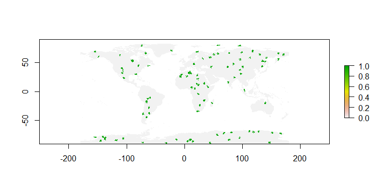 Then, we will
restrict the distribution of our species to these suitable habitat
patches:
Then, we will
restrict the distribution of our species to these suitable habitat
patches:
# Converting to a terra object
suitable.habitat <- rast(suitable.habitat)
my.sp3 <- limitDistribution(my.first.species,
                            geographical.limit = "raster",
                            area = suitable.habitat)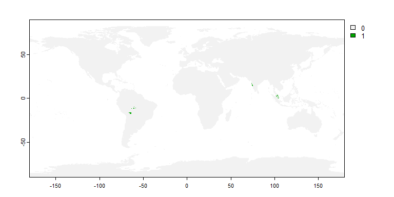
8.3. Sampling occurrence points in the dispersal-limited distribution
Once the distribution of a species has been limited with
limitDistribution(), you just have to apply
sampleOccurrences on this species: it will automatically
sample from the realised distribution of the species.
my.first.species <- limitDistribution(my.first.species,
                                      geographical.limit = "continent",
                                      area = "South America",
                                      plot = FALSE)

sampleOccurrences(my.first.species, n = 30)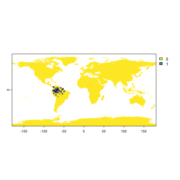
## Occurrence points sampled from a virtual species
##
## - Type: presence only
## - Number of points: 30
## - No sampling bias
## - Detection probability:
##    .Probability: 1
##    .Corrected by suitability: FALSE
## - Probability of identification error (false positive): 0
## - Multiple samples can occur in a single cell: No
##
## First 10 lines:
##                 x         y Real Observed
## 1195117 -73.91667 -2.250000    1        1
## 1223215 -70.91667 -4.416667    1        1
## 1249145 -69.25000 -6.416667    1        1
## 1186466 -75.75000 -1.583333    1        1
## 1143321 -66.58333  1.750000    1        1
## 1186507 -68.91667 -1.583333    1        1
## 1279348 -75.41667 -8.750000    1        1
## 1097960 -66.75000  5.250000    1        1
## 1192939 -76.91667 -2.083333    1        1
## 1195108 -75.41667 -2.250000    1        1
## ... 20 more lines.
-----------------
Do not hesitate if you have a question, find a bug, or would like to add a feature in virtualspecies: mail me!