5. Generating random species
The virtualspecies package embeds a function to randomly
generate virtual species generateRandomSp, with many
customisable options to constrain the randomisation process.
Let’s take a look:
library(virtualspecies)## Le chargement a nécessité le package : terra## terra 1.7.46## The legacy packages maptools, rgdal, and rgeos, underpinning the sp package,
## which was just loaded, will retire in October 2023.
## Please refer to R-spatial evolution reports for details, especially
## https://r-spatial.org/r/2023/05/15/evolution4.html.
## It may be desirable to make the sf package available;
## package maintainers should consider adding sf to Suggests:.
## The sp package is now running under evolution status 2
## (status 2 uses the sf package in place of rgdal)library(geodata)
worldclim <- worldclim_global(var = "bio", res = 10,
path = tempdir())
names(worldclim) <- paste0("bio", 1:19)
my.stack <- worldclim[[c("bio2", "bio5", "bio6", "bio12", "bio13", "bio14")]]
random.sp <- generateRandomSp(my.stack)## Reading raster values. If it fails for very large rasters, use arguments 'sample.points = TRUE' and define a number of points to sample with 'nb.point'.## - Perfoming the pca## - Defining the response of the species along PCA axes## - Calculating suitability values## The final environmental suitability was rescaled between 0 and 1.
## To disable, set argument rescale = FALSE## - Converting into Presence - Absence## --- Generating a random value of beta for the logistic conversion## --- Determing species.prevalence automatically according to alpha and beta## Logistic conversion finished:
##
## - beta = 0.807807807807808
## - alpha = -0.1
## - species prevalence =0.619959334350593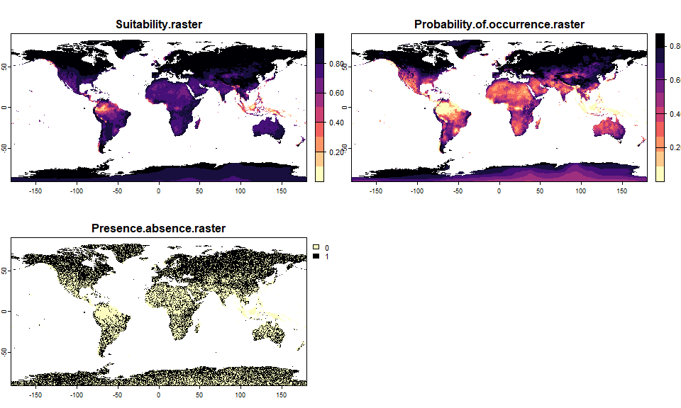
generateRandomSprandom.sp## Virtual species generated from 6 variables:
## bio2, bio5, bio6, bio12, bio13, bio14
##
## - Approach used: Response to axes of a PCA
## - Axes: 1, 2 ; 84.09 % explained by these axes
## - Responses to axes:
## .Axis 1 [min=-18.29; max=2.89] : dnorm (mean=0.2016541; sd=3.903569)
## .Axis 2 [min=-11.39; max=3.27] : dnorm (mean=-0.4790539; sd=3.738719)
## - Environmental suitability was rescaled between 0 and 1
##
## - Converted into presence-absence:
## .Method = probability
## .probabilistic method = logistic
## .alpha (slope) = -0.1
## .beta (inflexion point) = 0.807807807807808
## .species prevalence = 0.619959334350593We can see that the species was generated using a PCA approach.
Indeed, as
explained in the PCA section, when you have a lot of variables, it
becomes very difficult to generate a species with realistic
environmental requirements. Hence, by default the function
generateRandomSp uses a PCA approach if you have 6 or more
variables, and a ‘response functions’ approach if you have less than 6
variables.
In the next sections I detail the many possible customisations for
the function generateRandomSp.
5.1. General parameters
5.1.1. Choosing the approach
You can choose approach =:
"automatic": a ‘response’ approach is used if you have less than 6 variables and a ‘PCA’ approach is used if you have 6 or more variables"random": a random approach is chosen (response or PCA)"response": to use a response approach"pca": to use a pca approach
5.1.2. Rescaling of the environmental suitability
By default, rescale = TRUE, which means that the
environmental suitability is rescaled between 0 and 1.
5.1.3. Conversion to presence-absence
You can choose to enable the conversion of environmental suitability
to presence-absence. To do this, set convert.to.PA = TRUE.
You can customise the conversion:
- choose the conversion method with
PA.method. You should leave it toprobabilityunless you have a very particular reason to use thethresholdapproach. - define the parameters
alpha,betaandspecies.prevalenceexactly as explained in the convert to presence-absence section, or leave them as they are to create a random conversion into presence-absence
5.2. Parameters specific to a ‘response’ approach
5.2.1. Define the possible response functions
At the moment, four relations are possible for a random generation of
virtual species: Gaussian (gaussian), linear
(linear), logistic (logistic) and quadratic
(quadratic) relations. By default, all the relation types
are used. You can choose to use any combination with the argument
relations:
# A species with gaussian and logistic response functions
random.sp1 <- generateRandomSp(worldclim[[1:3]],
                              relations = c("gaussian", "logistic"),
                              convert.to.PA = FALSE)
## - Determining species' response to predictor variables## - Calculating species suitability## Generating virtual species environmental suitability...## - The response to each variable was rescaled between 0 and 1. To
## disable, set argument rescale.each.response = FALSE## - The final environmental suitability was rescaled between 0 and 1. To disable, set argument rescale = FALSE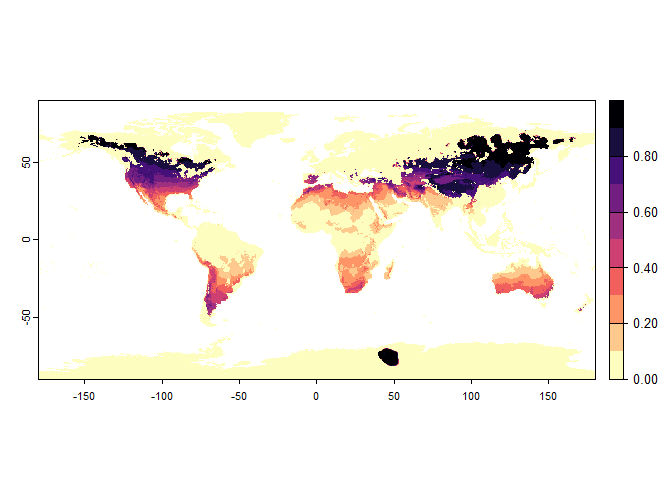
generateRandomSp, with gaussian and logistic response
functionsrandom.sp1## Virtual species generated from 3 variables:
## bio1, bio2, bio3
##
## - Approach used: Responses to each variable
## - Response functions:
## .bio1 [min=-54.72435; max=30.98764] : logisticFun (alpha=8.57119941711426; beta=21.8711321403201)
## .bio2 [min=1; max=21.14754] : logisticFun (alpha=-0.0422950820922852; beta=11.1666318553907)
## .bio3 [min=9.131122; max=100] : dnorm (mean=8.29268228976845; sd=81.3831553774217)
## - Each response function was rescaled between 0 and 1
## - Environmental suitability formula = bio1 * bio2 * bio3
## - Environmental suitability was rescaled between 0 and 1plotResponse(random.sp1)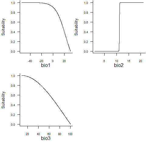
# A purely gaussian species
random.sp2 <- generateRandomSp(worldclim[[1:3]],
                              relations = "gaussian",
                              convert.to.PA = FALSE)
## - Determining species' response to predictor variables## - Calculating species suitability## Generating virtual species environmental suitability...## - The response to each variable was rescaled between 0 and 1. To
## disable, set argument rescale.each.response = FALSE## - The final environmental suitability was rescaled between 0 and 1. To disable, set argument rescale = FALSE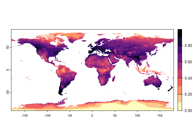
generateRandomSp, with gaussian response functions
onlyrandom.sp2## Virtual species generated from 3 variables:
## bio2, bio1, bio3
##
## - Approach used: Responses to each variable
## - Response functions:
## .bio2 [min=1; max=21.14754] : dnorm (mean=9.82209201879464; sd=16.0716527336248)
## .bio1 [min=-54.72435; max=30.98764] : dnorm (mean=4.45951290361598; sd=26.2632747667275)
## .bio3 [min=9.131122; max=100] : dnorm (mean=49.4464944649446; sd=70.2257022570226)
## - Each response function was rescaled between 0 and 1
## - Environmental suitability formula = bio2 * bio1 * bio3
## - Environmental suitability was rescaled between 0 and 1plotResponse(random.sp2)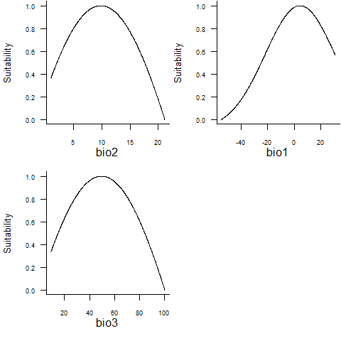
5.2.2. Rescale individual response functions
As explained in the section on the ‘response’ approach, you can
choose to rescale or not each individual response function, with the
argument rescale.each.response. TRUE by
default.
5.2.3. Try to find a realistic species
An important issue with the generation of random responses to the
environment, is that you can obtain a species willing to live in summer
temperatures of 35°C and winter temperature of -50°C. This may
interesting for generating species from another planet, but you are
probably more interested in generating species that can actually live on
Earth. There is therefore an option to do that, activated by default:
realistic.sp.
When activating this argument, the function will proceed step-by-step to try defining a realistic species. At step one, one of the variable is chosen, and the program randomly determines a response function for this variable. Then, it will compute the environmental suitability of this species. At step two, the program will pick a second variable, and will constrain its random generation depending on the environmental suitability obtained at step one. For example, if at step 2 a gaussian response is picked, then the mean will be chosen in areas where the species had a high environmental suitability. Then, the environmental suitability is recalculated on the basis of the first two response functions. At step 3, another variable is picked, a response function randomly generated with respect to areas where the species already has a high suitability, and so on until there are no variables left. While this process can help, it does not always work, and can provide completely unrealistic results also. In this case, you should try different runs, or switch to a ‘PCA’ approach.
Let’s see an example :
realistic.sp <- generateRandomSp(worldclim[[c(1, 5)]],
                                 realistic.sp = TRUE,
                                 convert.to.PA = FALSE)
## - Determining species' response to predictor variables## - Calculating species suitability## Generating virtual species environmental suitability...## - The response to each variable was rescaled between 0 and 1. To
## disable, set argument rescale.each.response = FALSE## - The final environmental suitability was rescaled between 0 and 1. To disable, set argument rescale = FALSE
unrealistic.sp <- generateRandomSp(worldclim[[c(1, 5)]],
                                   realistic.sp = FALSE,
                                   convert.to.PA = FALSE)
## - Determining species' response to predictor variables## - Calculating species suitability## Generating virtual species environmental suitability...## - The response to each variable was rescaled between 0 and 1. To
## disable, set argument rescale.each.response = FALSE## - The final environmental suitability was rescaled between 0 and 1. To disable, set argument rescale = FALSE
Note that you can always let the function randomly determine the
conversion to presence-absence by changing the argument
convert.to.PA = TRUE (be careful: since parameters are
defined randomly, the results can be bizarre), or you can do it by
yourself later:
realistic.sp <- convertToPA(realistic.sp, beta = 0.5) ## --- Determing species.prevalence automatically according to alpha and beta## Logistic conversion finished:
##
## - beta = 0.5
## - alpha = -0.05
## - species prevalence =0.0611680174444003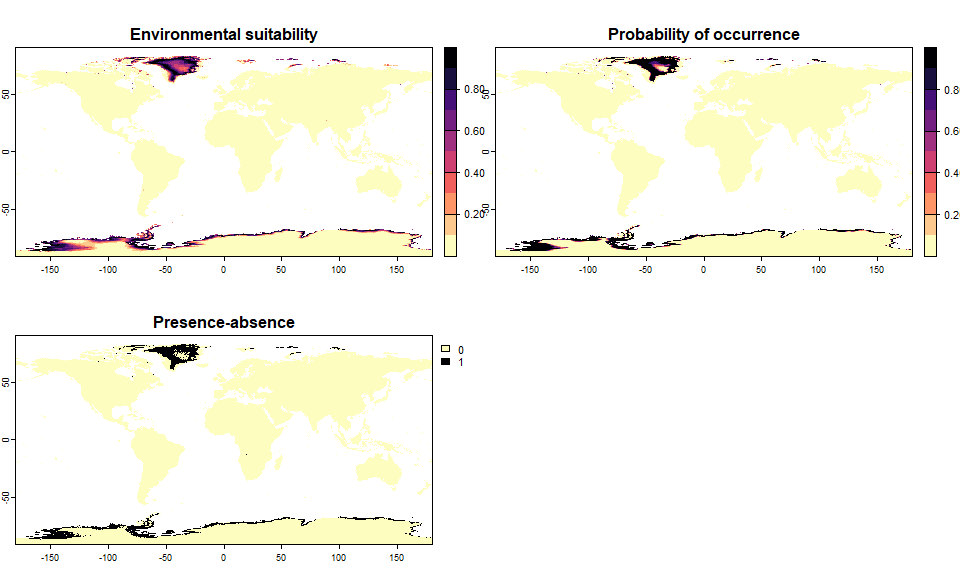
If, in spite of all your attempts, you are struggling to obtain satisfactory species, then perhaps you should try the ‘PCA’ approach.
5.2.4. Define how response functions are combined to compute the
environmental suitability
You can define how response functions are combined with the argument
sp.type, exactly as explained in the ‘response’ approach
section:
species.type = "additive": the response functions are added.species.type = "multiplicative": the response functions are multiplied (default value).species.type = "mixed": there is a mix of additions and products to calculate the environmental suitability, randomly generated.
5.3. Parameters specific to a ‘PCA’ approach
5.3.1. Generate a random species with a PCA approach on a low-memory
computer
As explained in the PCA section, if you have low-memory computer, or are working with very large raster files (large extent, fine resolution), then you can still perform the PCA by using a sample of the pixels of your raster.
To do this, set sample.points = TRUE, and choose the
number of pixels to sample, depending on your computer’s memory, with
nb.points.
# A safe run for a low memory computer
safe.run.sp <- generateRandomSp(worldclim[[c(1, 5, 6)]],
                                sample.points = TRUE,
                                nb.points = 1000)
## - Determining species' response to predictor variables## - Calculating species suitability## Generating virtual species environmental suitability...## - The response to each variable was rescaled between 0 and 1. To
## disable, set argument rescale.each.response = FALSE## - The final environmental suitability was rescaled between 0 and 1. To disable, set argument rescale = FALSE## - Converting into Presence - Absence## --- Generating a random value of beta for the logistic conversion## --- Determing species.prevalence automatically according to alpha and beta## Logistic conversion finished:
##
## - beta = 0.965965965965966
## - alpha = -0.1
## - species prevalence =0.0863161203534917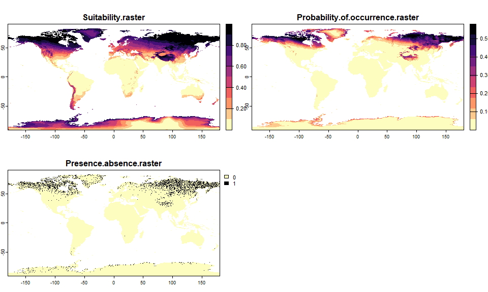
5.3.2. Generate stenotopic or eurytopic species
You can modify the niche.breadth argument to generate
stenotopic (niche.breadth = 'narrow'), eurytopic
(niche.breadth = 'wide'), or any type of species
(niche.breadth = 'any').
-----------------
Do not hesitate if you have a question, find a bug, or would like to add a feature in virtualspecies: mail me!