6. Exploring virtual species
This section is mainly intended to users not very familiar with R. For example, if you are not sure how to obtain the maps of generated virtual species, read this section. If you simply want to extract (sample) occurrence points for your virtual species, then you should jump to the next section.
6.1. Consult the details of a generated virtual species
Let’s create a simple virtual species:
library(virtualspecies)## Le chargement a nécessité le package : terra## terra 1.7.46## The legacy packages maptools, rgdal, and rgeos, underpinning the sp package,
## which was just loaded, will retire in October 2023.
## Please refer to R-spatial evolution reports for details, especially
## https://r-spatial.org/r/2023/05/15/evolution4.html.
## It may be desirable to make the sf package available;
## package maintainers should consider adding sf to Suggests:.
## The sp package is now running under evolution status 2
## (status 2 uses the sf package in place of rgdal)library(geodata)
# Worldclim data
worldclim <- worldclim_global(var = "bio", res = 10,
path = tempdir())
names(worldclim) <- paste0("bio", 1:19)
# Formatting of the response functions
my.parameters <- formatFunctions(bio1 = c(fun = 'dnorm', mean = 25, sd = 5),
bio12 = c(fun = 'dnorm', mean = 4000, sd = 2000))
# Generation of the virtual species
my.species <- generateSpFromFun(raster.stack = worldclim[[c("bio1", "bio12")]],
parameters = my.parameters)## Generating virtual species environmental suitability...## - The response to each variable was rescaled between 0 and 1. To
## disable, set argument rescale.each.response = FALSE## - The final environmental suitability was rescaled between 0 and 1. To disable, set argument rescale = FALSE# Conversion to presence-absence
my.species <- convertToPA(my.species,
beta = 0.7)## --- Determing species.prevalence automatically according to alpha and beta## Logistic conversion finished:
##
## - beta = 0.7
## - alpha = -0.05
## - species prevalence =0.024759514536794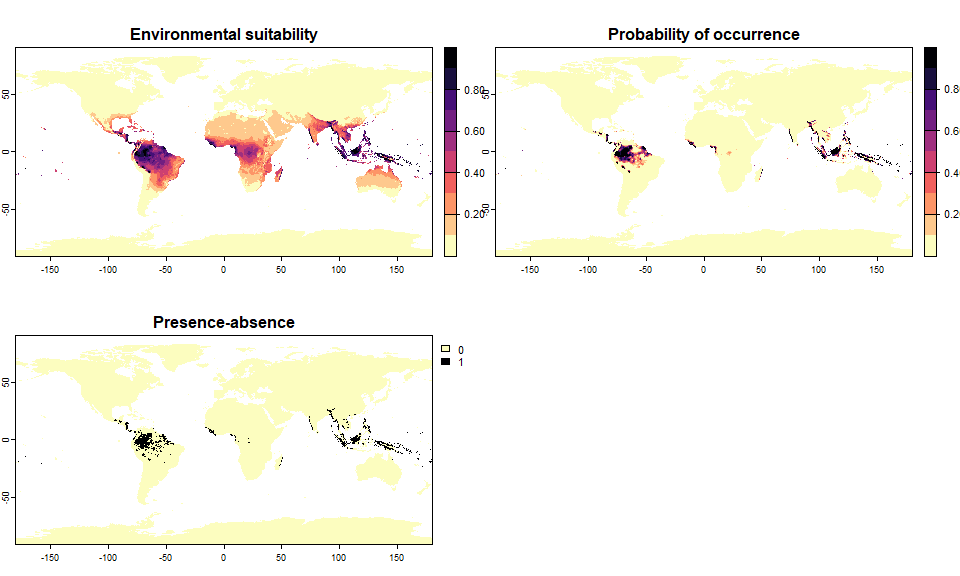
If we want to know how it was generated, we simply type the object name in the R console:
my.species## Virtual species generated from 2 variables:
## bio1, bio12
##
## - Approach used: Responses to each variable
## - Response functions:
## .bio1 [min=-54.72435; max=30.98764] : dnorm (mean=25; sd=5)
## .bio12 [min=0; max=11191] : dnorm (mean=4000; sd=2000)
## - Each response function was rescaled between 0 and 1
## - Environmental suitability formula = bio1 * bio12
## - Environmental suitability was rescaled between 0 and 1
##
## - Converted into presence-absence:
## .Method = probability
## .probabilistic method = logistic
## .alpha (slope) = -0.05
## .beta (inflexion point) = 0.7
## .species prevalence = 0.024759514536794And a summary of how the virtual species was generated appears:
- It shows us the variables used.
- It shows us the approach used and all the details of the approach, so we can use it to reconstruct another virtual species with the exact same parameters later on. It also provides us the range of values of our environmental variables (bio1 (mean annual temperature) ranged from -54.72°C to 30.99°C). This is helpful to quickly get an idea of the preferences of our species; for example here we see that we have a species living in hot environments, with a peak at 25°C.
- If a conversion to presence-absence was performed, it shows us the parameters of the conversion, and provides the species prevalence (the species prevalence is always calculated and provided).
- If you have introduced a distribution bias (will be seen in a later section), it will provide information about this particular bias.
6.2. Plot the virtual species map
Plotting the distribution maps of a virtual species is straightforward:
plot(my.species)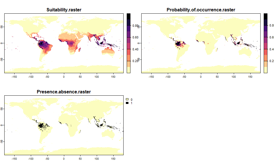
plot() on virtual species objectsIf the environmental suitability has been converted into presence-absence, then the plot will conveniently display both the environmental suitability and the presence-absence map.
6.3. Plot the species-environment relationship
As illustrated several times in this tutorial, there is a function to
automatically generate an appropriate plot for your virtual species:
plotResponse
plotResponse(my.species)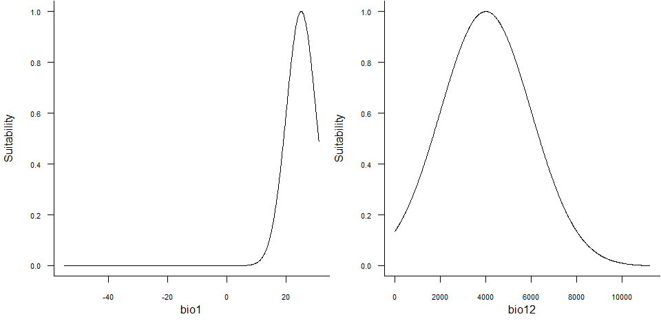
plotResponse() on a virtual species object6.4. Plot the relationship between suitability and probability of occurrence
If you converted your environmental suitability into presence-absence
with a probabilistic approach, chances are that you modified the
environmental suitability function, e.g. if you used a logistic method
or if you wanted to reach a specific prevalence. You may be interested
in the relationship between environmental suitability and probability of
occurrence, which can be plotted with
plotSuitabilityToProba
plotSuitabilityToProba(my.species)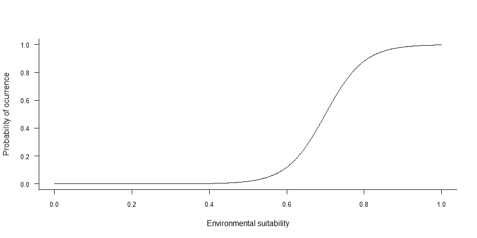
plotSuitabilityToProba() on a virtual species object6.5. Extracting elements of the virtual species, such as the rasters of environmental suitability
The virtual species object is structured as a list in R,
which roughly means that it is an object containing many “sub-objects”.
When you run functions on your virtual species object, such as the
conversion into presence-absence, then new sub-objects are added or
replaced in the list.
There is a function allowing you to see the content of the list:
str()
str(my.species)## List of 6
## $ approach : chr "response"
## $ details :List of 5
## ..$ variables : chr [1:2] "bio1" "bio12"
## ..$ formula : chr "bio1 * bio12"
## ..$ rescale.each.response: logi TRUE
## ..$ rescale : logi TRUE
## ..$ parameters :List of 2
## $ suitab.raster :S4 class 'SpatRaster' [package "terra"]
## $ PA.conversion : Named chr [1:5] "probability" "logistic" "-0.05" "0.7" ...
## ..- attr(*, "names")= chr [1:5] "conversion.method" "probabilistic.method" "alpha" "beta" ...
## $ probability.of.occurrence:S4 class 'SpatRaster' [package "terra"]
## $ pa.raster :S4 class 'SpatRaster' [package "terra"]
## - attr(*, "class")= chr [1:2] "virtualspecies" "list"We are informed that the object is a list containing 5
elements (sub-objects), that you can read on the lines starting with a
$: approach, details,
suitab.raster, PA.conversion and
pa.raster.
You can extract each element using the $: for example,
to extract the suitability raster, type
my.species$suitab.raster## class : SpatRaster
## dimensions : 1080, 2160, 1 (nrow, ncol, nlyr)
## resolution : 0.1666667, 0.1666667 (x, y)
## extent : -180, 180, -90, 90 (xmin, xmax, ymin, ymax)
## coord. ref. : lon/lat WGS 84 (EPSG:4326)
## source(s) : memory
## name : VSP suitability
## min value : 0
## max value : 1If you are interested in the probability of occurrence raster, type
my.species$probability.of.occurrence## class : SpatRaster
## dimensions : 1080, 2160, 1 (nrow, ncol, nlyr)
## resolution : 0.1666667, 0.1666667 (x, y)
## extent : -180, 180, -90, 90 (xmin, xmax, ymin, ymax)
## coord. ref. : lon/lat WGS 84 (EPSG:4326)
## source(s) : memory
## name : lyr.1
## min value : 8.315280e-07
## max value : 9.975274e-01If you are interested in the presence-absence raster, type
my.species$pa.raster## class : SpatRaster
## dimensions : 1080, 2160, 1 (nrow, ncol, nlyr)
## resolution : 0.1666667, 0.1666667 (x, y)
## extent : -180, 180, -90, 90 (xmin, xmax, ymin, ymax)
## coord. ref. : lon/lat WGS 84 (EPSG:4326)
## source(s) : memory
## name : lyr.1
## min value : 0
## max value : 1Technical note: rasters are terra objects which a stored in a
special format, called ‘wrapped format’, to ensure that these objects
can be safely saved to the disk for reproducibility. When you extract
these rasters from virtualspecies objects with $ or
[[ ]], they are silently unwrapped so that there is no
difference for the users.
You can also see that we have “sub-sub-objects”, in the lines
starting with ..$: these are objects contained within the
sub-object details. You can also extract them easily:
my.species$details$variables## [1] "bio1" "bio12"However, the sub-sub-sub-objects (level 3 of depth and beyond) are
not listed when you use str() on the entire virtual species
object. For example, if we extract the parameters object
from the details, we can see that it contains all the function names and
their parameters:
my.species$details$parameters## $bio1
## $bio1$fun
## fun
## "dnorm"
##
## $bio1$args
## mean sd
## 25 5
##
## $bio1$min
## [1] -54.72435
##
## $bio1$max
## [1] 30.98764
##
##
## $bio12
## $bio12$fun
## fun
## "dnorm"
##
## $bio12$args
## mean sd
## 4000 2000
##
## $bio12$min
## [1] 0
##
## $bio12$max
## [1] 11191# Looking at how it is structured:
str(my.species$details$parameters)## List of 2
## $ bio1 :List of 4
## ..$ fun : Named chr "dnorm"
## .. ..- attr(*, "names")= chr "fun"
## ..$ args: Named num [1:2] 25 5
## .. ..- attr(*, "names")= chr [1:2] "mean" "sd"
## ..$ min : num -54.7
## ..$ max : num 31
## $ bio12:List of 4
## ..$ fun : Named chr "dnorm"
## .. ..- attr(*, "names")= chr "fun"
## ..$ args: Named num [1:2] 4000 2000
## .. ..- attr(*, "names")= chr [1:2] "mean" "sd"
## ..$ min : num 0
## ..$ max : num 11191Hence, the main message here is if you want to explore the content of
the virtual species object, use the function str(), look at
which sub-objects you are interested in, and extract them with
$.
6.6. Saving the virtual species objects for later use
If you want to save a virtual species object, you can save it on your
hard drive, using the R function saveRDS():
saveRDS(my.species, file = "MyVirtualSpecies.RDS")You can load it in a later session of R, using
readRDS():
my.species <- readRDS("MyVirtualSpecies.RDS")
-----------------
Do not hesitate if you have a question, find a bug, or would like to add a feature in virtualspecies: mail me!