4. Converting environmental suitability to presence-absence

4.1. Introduction: why should we avoid a threshold conversion?

What we did so far was defining the relationship between the species and its environment. It was the most important part, but what it provides us is a spatial distribution of the species’ environmental suitability, not a spatial distribution of the species’ presences/absences. Hence we now have to convert the environmental suitability into presence-absence.

The simplest approach, which was also the most widely used until 2014, consists in defining a threshold of environmental suitability, below which conditions are unsuitable, so absence is attributed; and above which conditions are suitable, so presence is attributed. However, you should avoid this approach which is inadequate (see Meynard et al. 2019 for a review):

Most importantly, this creates completely unrealistic species:
- Real species are often absent from areas of high suitability, because of factors acting at smaller spatial scales, such as biotic pressure (competition, predation), disturbances, stochastic events.
- Real species often occur in unsuitable areas, because of very particular conditions allowing their occurrence (microclimatic/microhabitat conditions, climatic refugia).
The threshold almost completely removes the previously defined relationship between the species and its environment. The gradual aspect is lost: the above-threshold part of the environmental gradient is always fully suitable, while the below-threshold part is always fully unsuitable.

So, how can we convert our environmental suitability into presence-absence without a threshold?

We use a probabilistic approach: the probability of getting a presence of the species in a given pixel is dependent on its suitability in that pixel. With the package, the probability of presence can be defined as a linear transformation of environmental suitability, or as a logistic transformation of environmental suitability.

## Le chargement a nécessité le package : terra

## terra 1.7.46

## The legacy packages maptools, rgdal, and rgeos, underpinning the sp package,
## which was just loaded, will retire in October 2023.
## Please refer to R-spatial evolution reports for details, especially
## https://r-spatial.org/r/2023/05/15/evolution4.html.
## It may be desirable to make the sf package available;
## package maintainers should consider adding sf to Suggests:.
## The sp package is now running under evolution status 2
##      (status 2 uses the sf package in place of rgdal)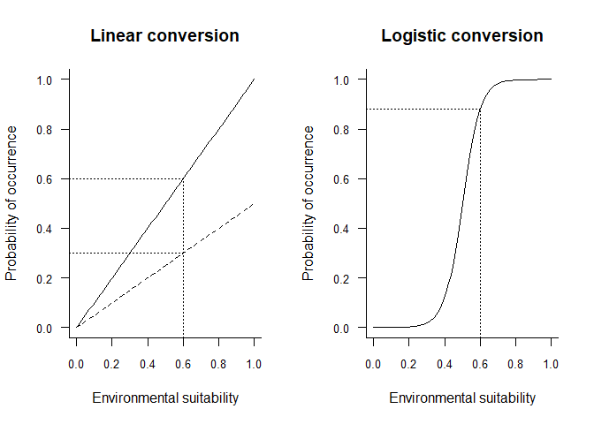

Fig. 4.1 Conversion of environmental suitability into probability of occurrence

In the example above, two linear conversions are illustrated (left panel), and one logistic conversion (right panel). The simplest method is to use environmental suitability as a probability of occurrence (left panel, plain line). In this case, a pixel with environmental suitability equal to 0.6 has 60% chance of having species presence, and 40% chance of having species absence. A linear conversion with a slope different from 1 may be chosen, e.g. to change the species prevalence (left panel, dashed line). In this example (slope = 0.5, intercept = 0), a pixel with environmental suitability equal to 0.6 has 30% chance of having species presence, and 70% chance of having species absence.

A logistic function on the other hand, will ensure that the simulated probability is within the 0-1 range and allow easycontrol of species prevalence. However, the logistic function will also flatten out the relationship at the extreme suitability values, and narrow or broaden the intermediate probability values depending on the slope of the logistic curve. In the example above (right panel), a pixel with environmental suitability equal to 0.6 has 88% chance of having species presence, and 12% chance of having species absence.

This means that we convert the environmental suitability of each pixel into a probability of occurrence. This probability of occurrence is then used to sample presence or absence in each cell, i.e., we make a random draw of presence or absence weighted by the probability of occurrence. As a consequence, repeated realisation of the presence-absence conversion will produce different occupancy maps, each providing a valid realisation of the true species distribution map.

The conversion is fully customisable, and can range from threshold conversion to logistic to linear conversion, by adjusting parameters (explained in section 4.2):

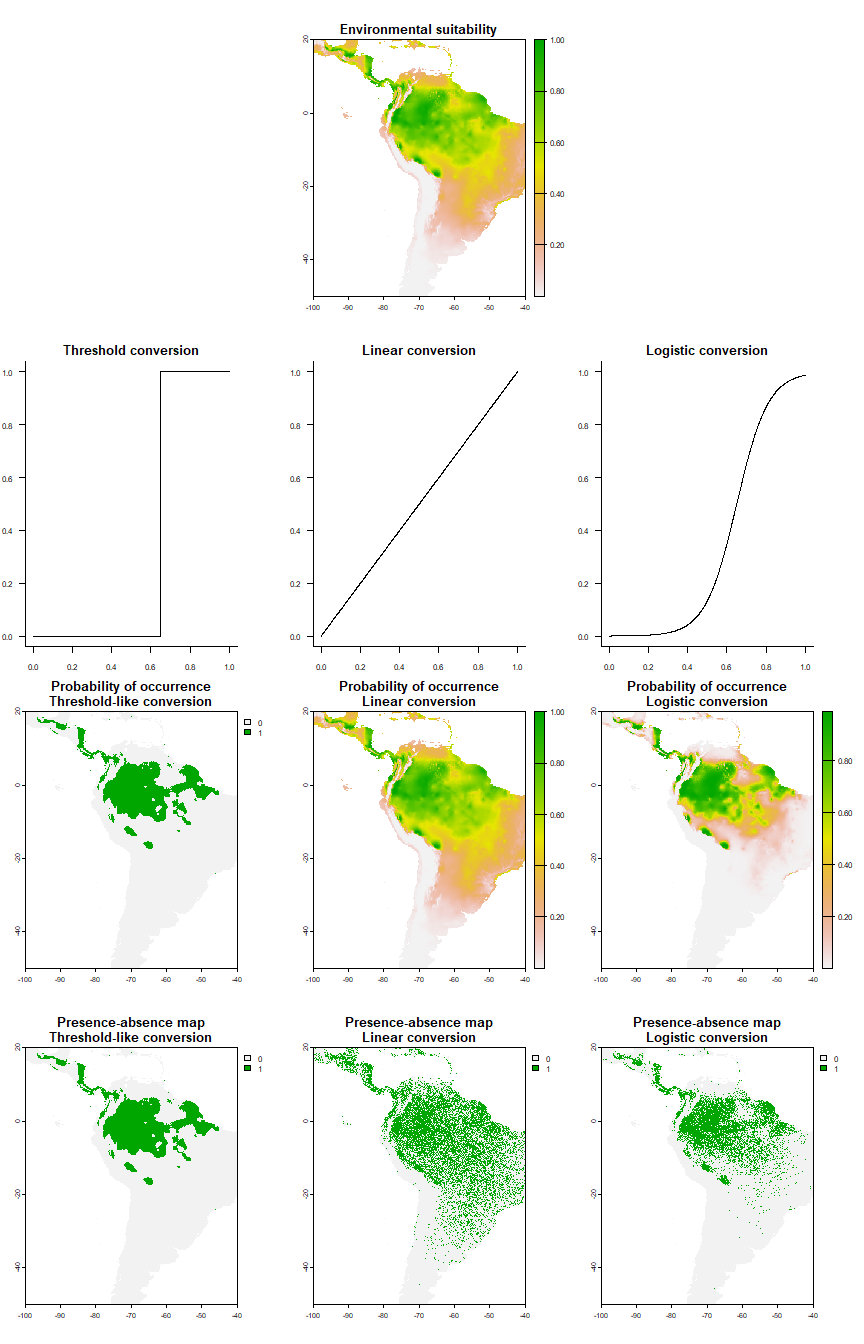
Fig. 4.2 Contrasting examples of conversion curves and their result on the distribution range of the same environmental suitability.

The logistic & linear conversions look much more realistic than the threshold-like conversion.

In the next section we will see how to perform the conversion, and how to customise it.

4.2. A quick example of the function in action

At first you may be interested to see the function in action, before we try to customise it. Here it is!

# Let's use the same species we generated before:
my.parameters <- formatFunctions(bio1 = c(fun = 'dnorm',
                                          mean = 25, sd = 5),
                                 bio12 = c(fun = 'dnorm',
                                           mean = 4000, sd = 2000))
my.first.species <- generateSpFromFun(raster.stack = worldclim[[c("bio1", "bio12")]],
                                      parameters = my.parameters,
                                      plot = FALSE)

# Run the conversion to presence-absence
pa1 <- convertToPA(my.first.species, plot = TRUE)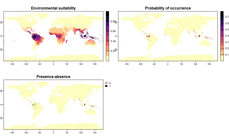

Fig. 4.3 Maps of environmental suitability and presence-absence of the virtual species

You have probably noticed that the conversion was performed without you choosing any parameter. This is because by default, the function performs a logistic conversion with random parameters. It would probably be better if you defined them yourself!

In the next section I summarise how to choose appropriate values of parameters, and then I illustrate how you can ask for a specific species prevalence (i.e., the number of places occupied by the species, out of the total number of available places) and let the function decide the parameters for you.

4.3. Customisation of the conversion

4.3.1. Threshold conversion

This conversion can be selected by defining argument PA.method = "threshold". The only parameter that can be customised in this kind of conversion is beta which determines the threshold of suitability above which the species is present and below which the species is absent.

pa2 <- convertToPA(my.first.species, PA.method = "threshold", beta = 0.65)

##    Threshold conversion finished:
##               
## - cutoff = 0.65
## - species prevalence =0.0297987879507904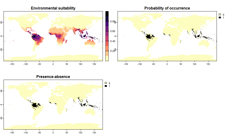

Fig. 4.4 Threshold conversion

4.3.2. Linear conversion

This conversion can be selected by defining arguments PA.method = "probability" (default value) and prob.method = "linear". Two arguments can be customised: the slope a and intercept b of the curve.

Here is a first example where the probability of occurrence is equal to environmental suitability:

pa3 <- convertToPA(my.first.species, PA.method = "probability",
                   prob.method = "linear", a = 1, b = 0)

##    --- Determing species prevalence automatically based
##                            on a linear transformation of environmental suitability of
##                            slope a = 1 and intercept b = 0

##    Linear conversion finished:
##               
## - slope (a) = 1
## - intercept (b) = 0
## - species prevalence =0.0866428315964423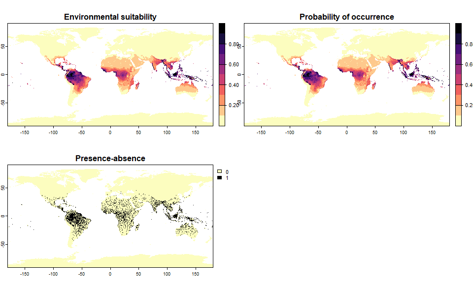

Fig. 4.5 Linear conversion

A second example where we change the probability of occurrence, which results in a difference in terms of species prevalence:

pa4 <- convertToPA(my.first.species, PA.method = "probability",
                   prob.method = "linear", a = 0.5, b = 0)

##    --- Determing species prevalence automatically based
##                            on a linear transformation of environmental suitability of
##                            slope a = 0.5 and intercept b = 0

##    Linear conversion finished:
##               
## - slope (a) = 0.5
## - intercept (b) = 0
## - species prevalence =0.0432558260411136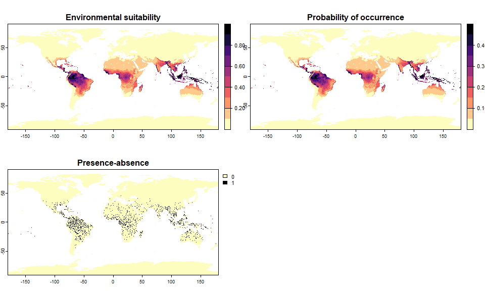

Fig. 4.6 Linear conversion

You can see the shape of the conversion with plotSuitabilityToProba:

plotSuitabilityToProba(pa3)
plotSuitabilityToProba(pa4, add = TRUE, lty = 2)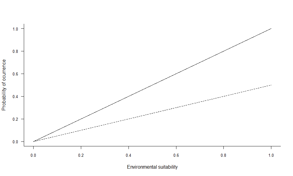

Fig. 4.7 Shapes of the conversion

4.3.3. Logistic conversion

This conversion can be selected by defining arguments PA.method = "probability" (default value) and prob.method = "logistic" (default value). The parameters \(\alpha\) (alpha) and \(\beta\) (beta)determine the shape of the logistic curve:

\(\beta\) controls the inflexion point,

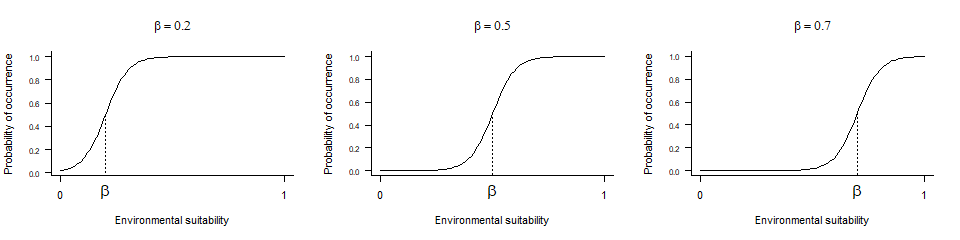
Fig. 4.8 Impact of beta on the conversion curve

and \(\alpha\) drives the ‘slope’ of the curve

Fig. 4.9 Impact of alpha on the conversion curve

The parameters are fairly simple to customise:

pa5 <- convertToPA(my.first.species,
                   PA.method = "probability",
                   prob.method = "logistic",
                   beta = 0.65, alpha = -0.07,
                   plot = TRUE)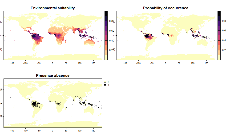

Fig. 4.10 Conversion with beta = 0.65, alpha = -0.07

# You can modify the conversion of your object if you did not like it:
pa5 <- convertToPA(pa5,
                   beta = 0.3, alpha = -0.02,
                   plot = TRUE)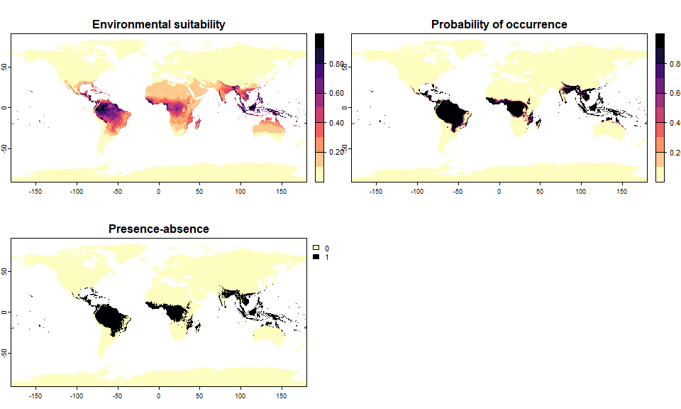

Fig. 4.11 Conversion with beta = 0.3, alpha = -0.02

plotSuitabilityToProba(pa5)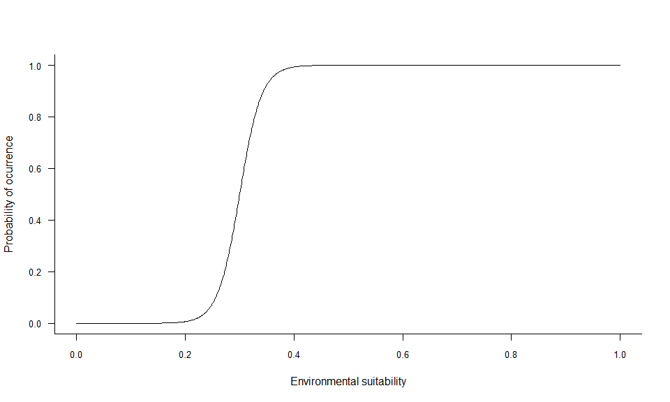

Fig. 4.12 Conversion of species pa5

4.3.3.1. beta

beta is very simple to grasp, as it is the inflexion point of the curve. Hence, looking at the three beta curves above, we can see that a lower beta will increase the probability of finding suitable conditions for the species (wider distribution range). A higher beta will decrease the probability of finding suitable conditions (smaller distribution range).

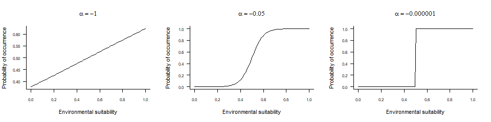
4.3.3.2. alpha

alpha may be more difficult to grasp, as it is dependent on the range of values of the x axis (in our case, the environmental suitability, ranging from 0 to 1):

If alpha is approximately equal to the range ofx or greater (in absolute value), then the conversion will have a linear shape. In our case, it means
values of alpha below -.3).
If alpha is about 5-10% of the range of x, then the conversion will be logistic. In our case, you can have nice logistic curves for values of alpha between -0.1 and -0.01.
If alpha is much smaller compared to x (in absolute value), then the conversion will be threshold-like. In our case, if means values of alpha in the range [-0.001, 0[.

4.4. Conversion to presence-absence based on a value of species prevalence

The species prevalence is the number of places (here, pixels) actually occupied by the species out of the total number of places (pixels) available. Do not confuse the SPECIES PREVALENCE with the SAMPLE PREVALENCE, which in turn is the proportion of samples in which you have found the species.

Numerous authors have shown the importance of the species prevalence in species distribution modelling, and how it can bias models. As a consequence, when generating virtual species distributions to test particular protocols or modelling techniques, you may be interested in testing different values of species prevalence. However, it is important to know that the species prevalence is dependent on the species-environment relationship, the shape of the probabilistic conversion curve AND the spatial distribution of environmental conditions. As a consequence, the function has to try different shapes of conversion curve to find a conversion according to your chosen value of species prevalence. Sometimes, it is not possible to reach a particular species prevalence, in that case the function will choose the conversion curve providing results closest to your species prevalence.

For all three types of conversion (threshold, linear, logistic), the function can automatically find parameters according to your chosen value of species prevalence.

4.4.1 Threshold conversion

In this case you just specify your value of species prevalence without any other parameter:

# Let's generate a species occupying 20% of the world
sp.0.2 <- convertToPA(my.first.species,
                      PA.method = "threshold",
                      species.prevalence = 0.2)

##    Threshold conversion finished:
##               
## - cutoff = 0.1362433482644
## - species prevalence =0.200000495017035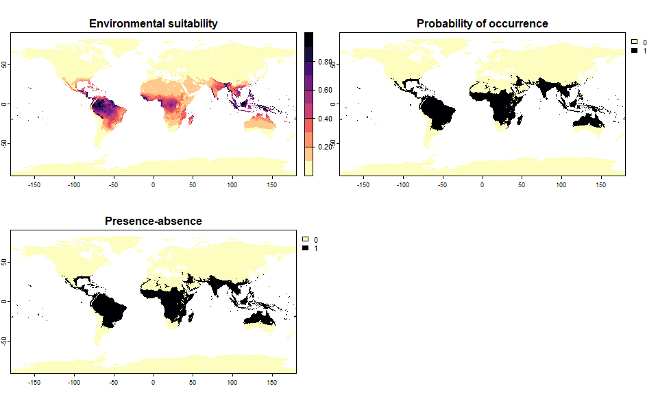

Fig. 4.13 Threshold conversion of a species with a prevalence of 0.2, i.e. occupying 20% of the world (which is quite large)

sp.0.2

## Virtual species generated from 2 variables:
##  bio1, bio12
## 
## - Approach used: Responses to each variable
## - Response functions:
##    .bio1  [min=-54.72435; max=30.98764] : dnorm   (mean=25; sd=5)
##    .bio12  [min=0; max=11191] : dnorm   (mean=4000; sd=2000)
## - Each response function was rescaled between 0 and 1
## - Environmental suitability formula = bio1 * bio12
## - Environmental suitability was rescaled between 0 and 1
## 
## - Converted into presence-absence:
##    .Method = threshold
##    .threshold           = 0.1362433482644
##    .species prevalence  = 0.200000495017035

4.4.2 Linear conversion

In this case again, you just specify your value of species prevalence without any other parameter, and the function will try to find a conversion that respects the chosen prevalence, and does not result in probabilities below 0 or above 1.

# Let's generate a species occupying 20% of the world
sp.0.2 <- convertToPA(my.first.species,
                      PA.method = "probability",
                      prob.method = "linear",
                      species.prevalence = 0.2)

##    --- Searching for a linear transformation of 
##                     environmental suitability that fits the chosen 
##                     species.prevalence.

##    Linear conversion finished:
##               
## - slope (a) = 0.876382668991938
## - intercept (b) = 0.123617331008062
## - species prevalence =0.200226965310444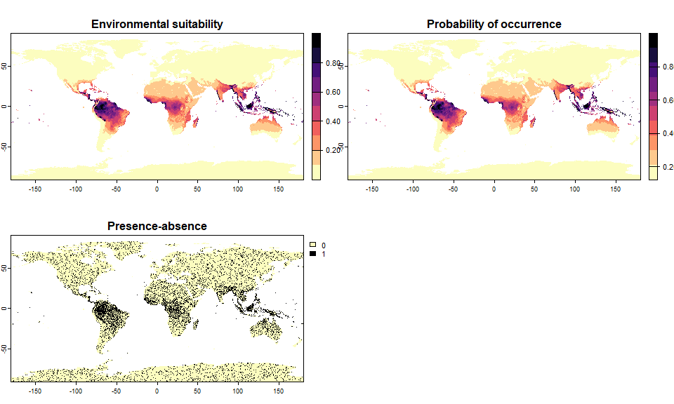

Fig. 4.14 Linear conversion of a species with a prevalence of 0.2

sp.0.2

## Virtual species generated from 2 variables:
##  bio1, bio12
## 
## - Approach used: Responses to each variable
## - Response functions:
##    .bio1  [min=-54.72435; max=30.98764] : dnorm   (mean=25; sd=5)
##    .bio12  [min=0; max=11191] : dnorm   (mean=4000; sd=2000)
## - Each response function was rescaled between 0 and 1
## - Environmental suitability formula = bio1 * bio12
## - Environmental suitability was rescaled between 0 and 1
## 
## - Converted into presence-absence:
##    .Method = probability
##    .probabilistic method    = linear
##    .a (slope)               = 0.876382668991938
##    .b (intercept)           = 0.123617331008062
##    .species prevalence      = 0.200226965310444

# And two others covering 5 and 50% of the world
sp.0.05 <- convertToPA(my.first.species,
                      PA.method = "probability",
                      prob.method = "linear",
                      species.prevalence = 0.05)

##    --- Searching for a linear transformation of 
##                     environmental suitability that fits the chosen 
##                     species.prevalence.

##    Linear conversion finished:
##               
## - slope (a) = 0.573679003730832
## - intercept (b) = 0
## - species prevalence =0.0499855826288622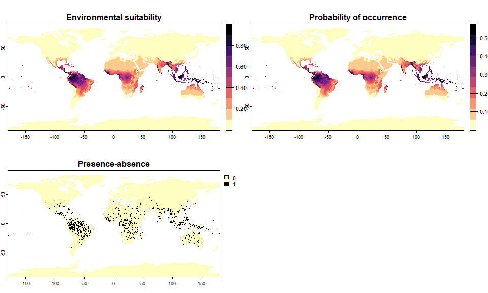

Fig. 4.15 Linear conversion of species with a prevalence 0.05 and 0.5

sp.0.5 <- convertToPA(my.first.species,
                      PA.method = "probability",
                      prob.method = "linear",
                      species.prevalence = 0.5)

##    --- Searching for a linear transformation of 
##                     environmental suitability that fits the chosen 
##                     species.prevalence.

##    Linear conversion finished:
##               
## - slope (a) = 0.547739168119961
## - intercept (b) = 0.452260831880039
## - species prevalence =0.499890477481056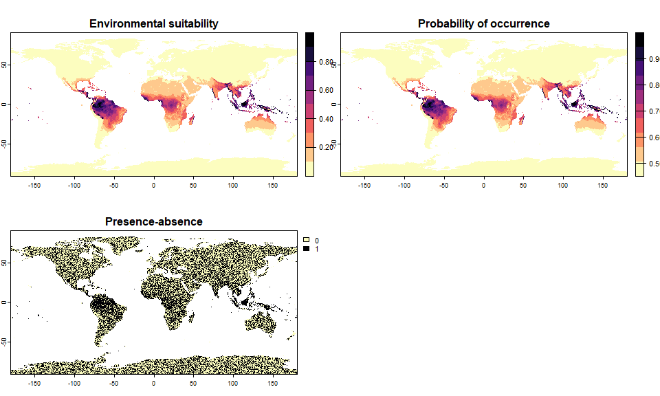

Fig. 4.15 Linear conversion of species with a prevalence 0.05 and 0.5

plotSuitabilityToProba(sp.0.05)
plotSuitabilityToProba(sp.0.2, add = TRUE, lty = 2)
plotSuitabilityToProba(sp.0.5, add = TRUE, lty = 3)
legend("topleft", lty = 1:3, legend = c(0.05, 0.2, 0.5), title = "Prevalence")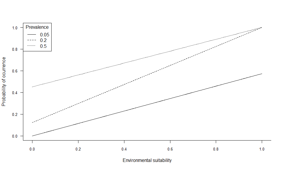

Fig. 4.16 Conversion of species pa5

4.4.3 Logistic conversion

For the logistic conversion, you have to fix either alpha or beta. I strongly advise to fix a value of alpha (this is the default parameter, with alpha = -0.05), so that the function will try to find an appropriate conversion by testing different values of beta. If you prefer to fix the value of beta, then the function will try different values of alpha, but it is likely that it will not be able to find a conversion generating a species with the appropriate prevalence.

Let’s see it in practice:

# Let's generate a species occupying 20% of the world
# Default settings, alpha = -0.05
sp.0.2 <- convertToPA(my.first.species,
                      species.prevalence = 0.2)

##    --- Determing beta automatically according to alpha and species.prevalence

##    Logistic conversion finished:
##               
## - beta = 0.17578125
## - alpha = -0.05
## - species prevalence =0.200578427405133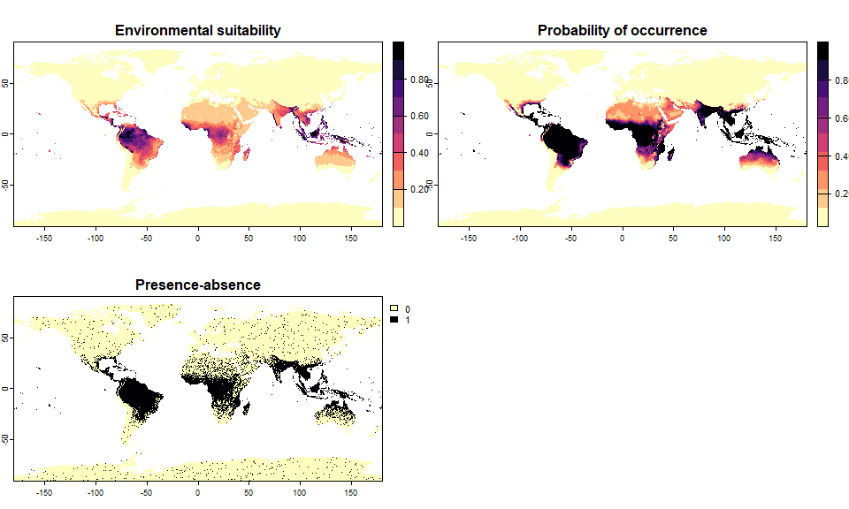

Fig. 4.17 Conversion of a species with a prevalence of 0.2, i.e. occupying 20% of the world (which is quite large)

sp.0.2

## Virtual species generated from 2 variables:
##  bio1, bio12
## 
## - Approach used: Responses to each variable
## - Response functions:
##    .bio1  [min=-54.72435; max=30.98764] : dnorm   (mean=25; sd=5)
##    .bio12  [min=0; max=11191] : dnorm   (mean=4000; sd=2000)
## - Each response function was rescaled between 0 and 1
## - Environmental suitability formula = bio1 * bio12
## - Environmental suitability was rescaled between 0 and 1
## 
## - Converted into presence-absence:
##    .Method = probability
##    .probabilistic method    = logistic
##    .alpha (slope)           = -0.05
##    .beta  (inflexion point) = 0.17578125
##    .species prevalence      = 0.200578427405133

# Now, a species occupying 1.5% of the world
# Change alpha to have a slightly more steep curve
sp.0.015 <- convertToPA(my.first.species,
                        species.prevalence = 0.015,
                        alpha = -0.015)

##    --- Determing beta automatically according to alpha and species.prevalence

##    Logistic conversion finished:
##               
## - beta = 0.78125
## - alpha = -0.015
## - species prevalence =0.0145052366614566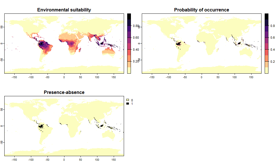

Fig. 4.18 Conversion of a species with a prevalence of 0.015, i.e. occupying 1.5% of the world

sp.0.015

## Virtual species generated from 2 variables:
##  bio1, bio12
## 
## - Approach used: Responses to each variable
## - Response functions:
##    .bio1  [min=-54.72435; max=30.98764] : dnorm   (mean=25; sd=5)
##    .bio12  [min=0; max=11191] : dnorm   (mean=4000; sd=2000)
## - Each response function was rescaled between 0 and 1
## - Environmental suitability formula = bio1 * bio12
## - Environmental suitability was rescaled between 0 and 1
## 
## - Converted into presence-absence:
##    .Method = probability
##    .probabilistic method    = logistic
##    .alpha (slope)           = -0.015
##    .beta  (inflexion point) = 0.78125
##    .species prevalence      = 0.0145052366614566

# Let's try by fixing beta rather than alpha
# We want a species occupying 10% of the world, with a high value of beta
sp.10 <- convertToPA(my.first.species,
                     species.prevalence = 0.1,
                     alpha = NULL,
                     beta = 0.9)

##    --- Determing alpha automatically according to beta and species.prevalence

##    Logistic conversion finished:
##               
## - beta = 0.9
## - alpha = -0.35252734375
## - species prevalence =0.100947586358816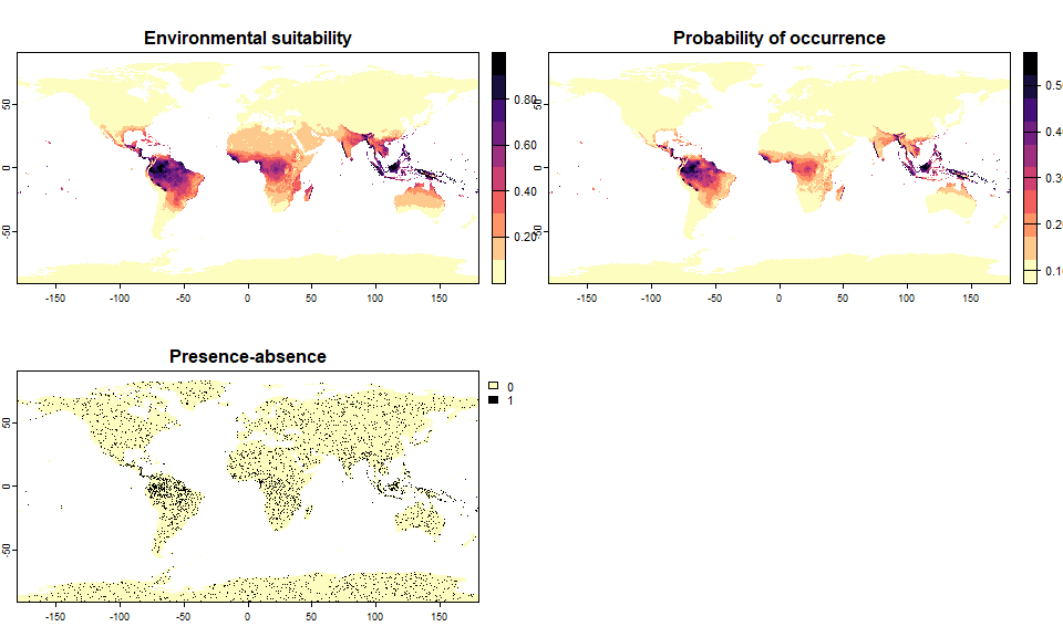

Fig. 4.19 Conversion of a species with a prevalence of 0.1, i.e. occupying 10% of the world

sp.10

## Virtual species generated from 2 variables:
##  bio1, bio12
## 
## - Approach used: Responses to each variable
## - Response functions:
##    .bio1  [min=-54.72435; max=30.98764] : dnorm   (mean=25; sd=5)
##    .bio12  [min=0; max=11191] : dnorm   (mean=4000; sd=2000)
## - Each response function was rescaled between 0 and 1
## - Environmental suitability formula = bio1 * bio12
## - Environmental suitability was rescaled between 0 and 1
## 
## - Converted into presence-absence:
##    .Method = probability
##    .probabilistic method    = logistic
##    .alpha (slope)           = -0.35252734375
##    .beta  (inflexion point) = 0.9
##    .species prevalence      = 0.100947586358816

It worked, but the resulting species does not look realistic at all: alpha was below -0.3, which means that we had a quasi-linear conversion curve, producing this unrealistic presence-absence map.

# Now an impossible task: a low value of beta for the same requirements:
sp.10bis <- convertToPA(my.first.species,
                        species.prevalence = 0.1,
                        alpha = NULL,
                        beta = 0.3)

##    --- Determing alpha automatically according to beta and species.prevalence

## Warning in convertToPA(my.first.species, species.prevalence = 0.1, alpha = NULL, : Warning, the desired species prevalence cannot be obtained, because of the chosen beta and available environmental conditions (see details).
##                           The closest possible estimate of prevalence was 0.11 
## Perhaps you can try a higher beta value.

##    Logistic conversion finished:
##               
## - beta = 0.3
## - alpha = -0.001
## - species prevalence =0.108688415240089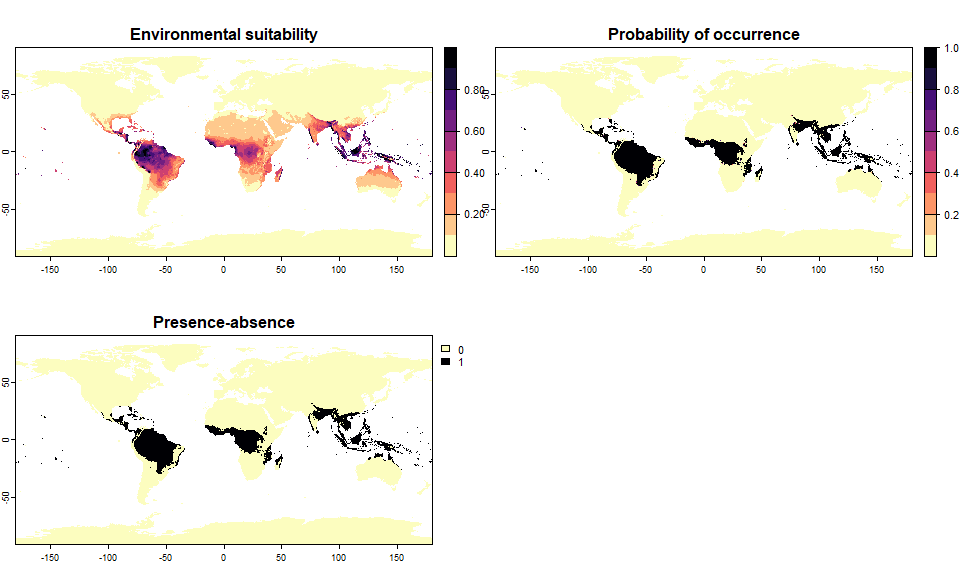

Fig. 4.20 Conversion of a species whose asked prevalence (0.1) cannot be reached because of a too low value of beta

sp.10bis

## Virtual species generated from 2 variables:
##  bio1, bio12
## 
## - Approach used: Responses to each variable
## - Response functions:
##    .bio1  [min=-54.72435; max=30.98764] : dnorm   (mean=25; sd=5)
##    .bio12  [min=0; max=11191] : dnorm   (mean=4000; sd=2000)
## - Each response function was rescaled between 0 and 1
## - Environmental suitability formula = bio1 * bio12
## - Environmental suitability was rescaled between 0 and 1
## 
## - Converted into presence-absence:
##    .Method = probability
##    .probabilistic method    = logistic
##    .alpha (slope)           = -0.001
##    .beta  (inflexion point) = 0.3
##    .species prevalence      = 0.108688415240089

Let’s see how the conversion curves look like:

plotSuitabilityToProba(sp.0.015)
plotSuitabilityToProba(sp.0.2, add = TRUE, lty = 2)
plotSuitabilityToProba(sp.10, add = TRUE, lty = 3)
plotSuitabilityToProba(sp.10bis, add = TRUE, lty = 4)
legend("topleft", lty = 1:4, legend = c(0.015, 0.2, 0.1, "0.1 (failed)"), title = "Prevalence")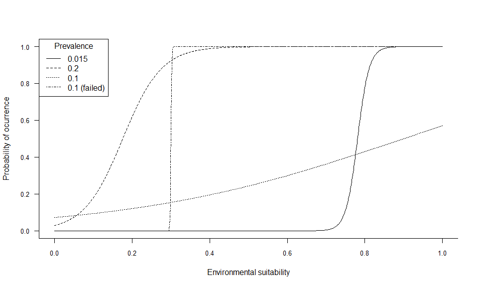

Fig. 4.21 Logistic conversions of species sp0.015, sp0.2, sp.10, sp.10bis

-----------------
Do not hesitate if you have a question, find a bug, or would like to add a feature in virtualspecies: mail me!