3. Virtual species defined by response to a PCA of the environment
If you try to use the “response” approach with a large number of variables, e.g. 10, then you will rapidly hit the unextricable problem of unrealistic environmental requirements. When you have 2 environmental variables, it is easy to choose response functions that are compatible. For example, you know that you should not try to generate a species which requires a temperature of the warmest month at 35°C, and a temperature of the coldest month at -25°C, because such conditions are unlikely to exist on Earth. However, if you have 10 variables, the task is much more complicated: if you want to generate a species which is dependent on 5 different temperature variables, 3 precipitation variables, and 2 land use variables, then it is almost impossible to know if your response functions are realistic regarding environmental conditions.
This is why we implemented the second approach, which consists in
generating a Principal Component Analysis (PCA) of all the environmental
variables in your SpatRaster, and then define the response
of the species to two axes (pricipal components). Using this approach
will greatly help you to generate virtual species which have plausible
environmental requirements, while being dependent on all of your
variables.
The function providing this approach is
generateSpFromPCA.
3.1. An introduction example
We want to generate a species dependent on three temperature variables (bio2, bio5 and bio6) and three precipitation variables (bio12, bio13, bio14 ).
library(geodata)## Le chargement a nécessité le package : terra## terra 1.7.46worldclim <- worldclim_global(var = "bio", res = 10,
path = tempdir())
# Rename bioclimatic variables for simplicity
names(worldclim) <- paste0("bio", 1:19)
my.stack <- worldclim[[c("bio2", "bio5", "bio6", "bio12", "bio13", "bio14")]]The generation of a virtual species is relatively straightforward:
library(virtualspecies)## The legacy packages maptools, rgdal, and rgeos, underpinning the sp package,
## which was just loaded, will retire in October 2023.
## Please refer to R-spatial evolution reports for details, especially
## https://r-spatial.org/r/2023/05/15/evolution4.html.
## It may be desirable to make the sf package available;
## package maintainers should consider adding sf to Suggests:.
## The sp package is now running under evolution status 2
## (status 2 uses the sf package in place of rgdal)my.pca.species <- generateSpFromPCA(raster.stack = my.stack)## Reading raster values. If it fails for very large rasters, use arguments 'sample.points = TRUE' and define a number of points to sample with 'nb.point'.## - Perfoming the pca## - Defining the response of the species along PCA axes## - Calculating suitability values## The final environmental suitability was rescaled between 0 and 1.
## To disable, set argument rescale = FALSE## Argument rescale was not specified, so it was automatically defined to TRUE. Verify that this is what you want.## No default value was defined for rescale.each.response, setting rescale.each.response = TRUE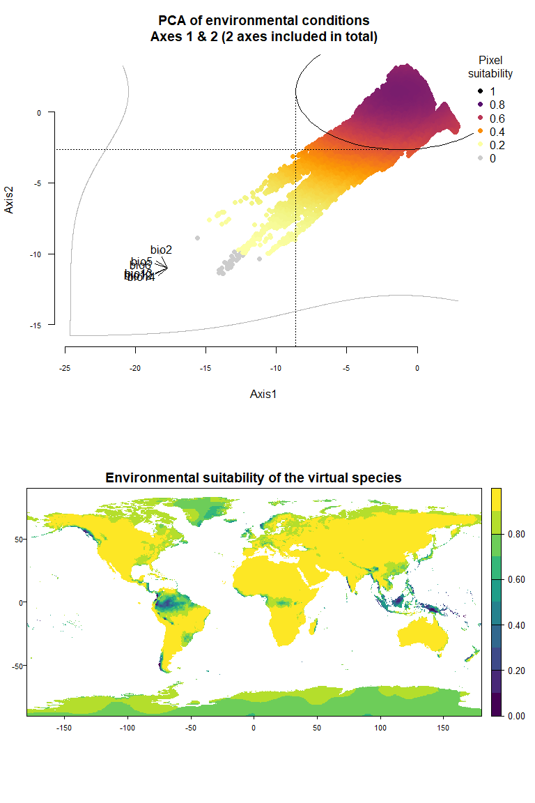
my.pca.species## Virtual species generated from 6 variables:
## bio2, bio5, bio6, bio12, bio13, bio14
##
## - Approach used: Response to axes of a PCA
## - Axes: 1, 2 ; 84.09 % explained by these axes
## - Responses to axes:
## .Axis 1 [min=-18.29; max=2.89] : dnorm (mean=-1.191869; sd=7.448132)
## .Axis 2 [min=-11.39; max=3.27] : dnorm (mean=1.419812; sd=4.0735)
## - Environmental suitability was rescaled between 0 and 1Something very important to know here is that the PCA is performed on
all the pixels of the raster stack. As a consequence, if you use large
stacks (large spatial scales, fine resolutions), your computer may not
be able to extract all the values. In this case, you can run the PCA on
a random subset of values, by setting sample.points = TRUE
and defining the number of pixels to sample with nb.points
(default 10000, try less if your computer is struggling).
my.pca.species <- generateSpFromPCA(raster.stack = my.stack,
                                    sample.points = TRUE, nb.points = 5000)
## - Perfoming the pca## - Defining the response of the species along PCA axes## - Calculating suitability values## The final environmental suitability was rescaled between 0 and 1.
## To disable, set argument rescale = FALSE## Argument rescale was not specified, so it was automatically defined to TRUE. Verify that this is what you want.## No default value was defined for rescale.each.response, setting rescale.each.response = TRUE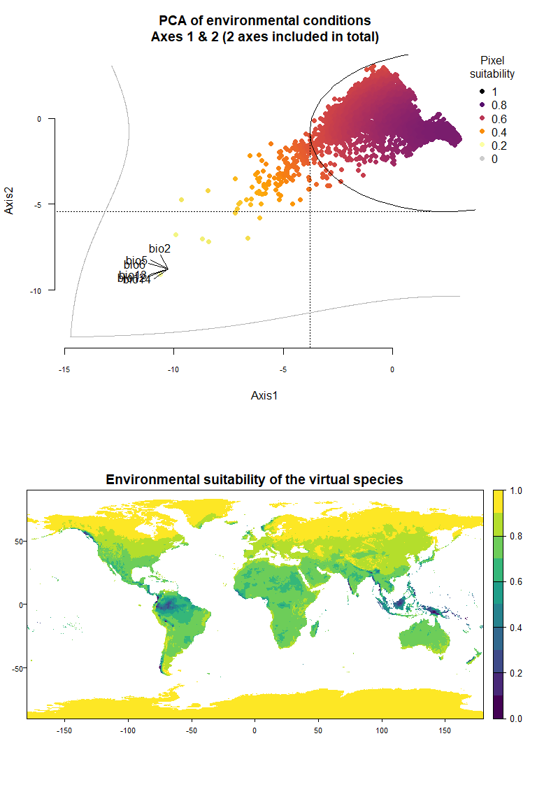
my.pca.species## Virtual species generated from 6 variables:
## bio2, bio5, bio6, bio12, bio13, bio14
##
## - Approach used: Response to axes of a PCA
## - Axes: 1, 2 ; 83.67 % explained by these axes
## - Responses to axes:
## .Axis 1 [min=-10.61; max=3.06] : dnorm (mean=2.48194; sd=6.265016)
## .Axis 2 [min=-9.1; max=3.06] : dnorm (mean=-0.7576087; sd=4.672329)
## - Environmental suitability was rescaled between 0 and 1Congratulations! You have just generated your first virtual species
with a PCA. You will probably have noticed that you have not entered any
parameter, but the generation has still succeeded. Indeed, when no
parameter is entered, the response of the species to PCA axes is
randomly generated. The reason behind this choice is that you can hardly
choose by yourself the parameters before you have seen the PCA! The next
step is therefore to take a look at the PCA, using the function
plotResponse (note that you can also use the argument
plot = TRUE in generateSpFromPCA)
plotResponse(my.pca.species)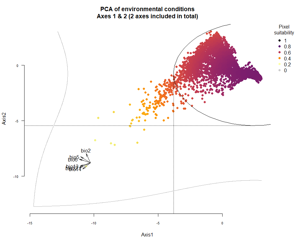
On Fig. 3.1 you can see the PCA of environmental conditions, where each point is the representation of a pixel of your stack in the factorial space. On one of the corners is shown the projection of the variables on this PCA (the position varies for an easier reading, although it is not always perfect). Along each axis, you can see the response of the species: its tolerance to the axis 1, driven mostly by precipitation variables (bio12, 13 and 14 bio13), and its tolerance to the axis 2, driven mostly by temperature variables (bio2 mostly, and bio5 & 6 to a lesser extent and bio5). The resulting environmental suitability, as a product of responses to each axis, is illustrated by a coloration of the points, from purple (high suitability), to yellow and grey (low/unsuitable pixels).
Now that you have this information in hand, you will be able (in the next section) to define a narrower niche breadth for the species, or to choose a species living in hotter, colder, drier or wetter environments. But before that, you probably would like to see how the species’ environmental suitability is distributed in space. Nothing’s simpler:
plot(my.pca.species)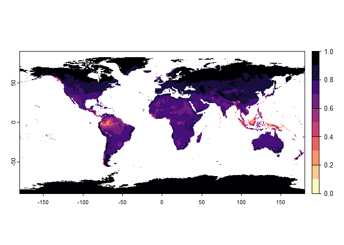
3.2. Customisation of the parameters
The function generateSpFromPCA proceeds into four
important steps: 1. The PCA is computed on the basis of the input
environmental conditions. You can also provide your own PCA. 2. The
Gaussian responses to axes are randomly chosen (only if you did not
provide precise parameters) and then computed. 3. The environmental
suitability is calculated as a product of the responses to both axes. 4.
The environmental suitability is rescaled between 0 and 1. This step can
be disabled.
3.2.1. Customisation of the responses to axes
You can customise the Gaussian response functions in two different ways:
- You can constrain the random generation of parameters by choosing
either a narrow-niche or a broad-niche species. To do this, specify the
argument
niche.breadth = 'narrow'orniche.breadth = 'wide'. By default this argument is set toniche.breadth = 'any', meaning that you can obtain species with any niche breadth.
This argument controls the standard deviation of the gaussian distribution. The full details about this is available in the help of the function (?generateSpFromPCA)
narrow.species <- generateSpFromPCA(raster.stack = my.stack,
                                    sample.points = TRUE,
                                    nb.points = 5000,
                                    niche.breadth = "narrow")
## - Perfoming the pca## - Defining the response of the species along PCA axes## - Calculating suitability values## The final environmental suitability was rescaled between 0 and 1.
## To disable, set argument rescale = FALSE## Argument rescale was not specified, so it was automatically defined to TRUE. Verify that this is what you want.## No default value was defined for rescale.each.response, setting rescale.each.response = TRUE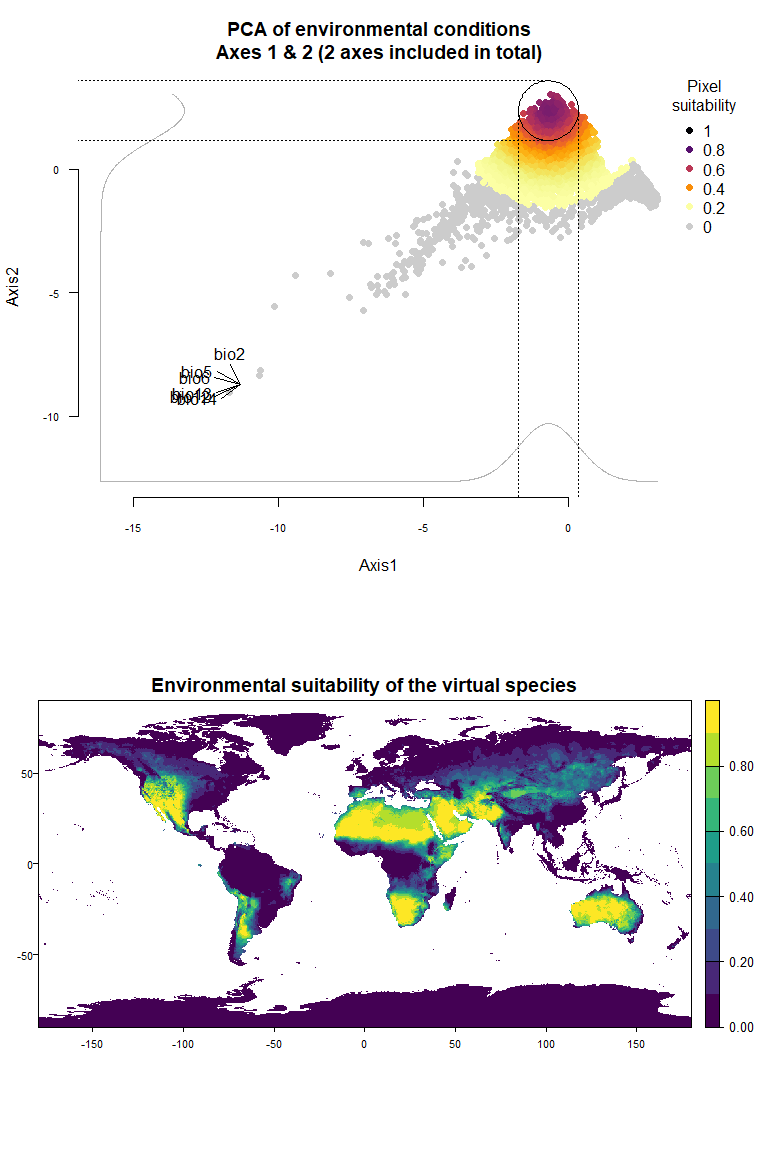
plotResponse(narrow.species)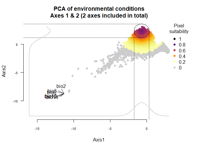
plot(narrow.species)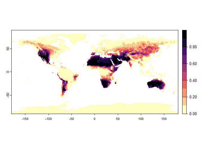
wide.species <- generateSpFromPCA(raster.stack = my.stack, sample.points = TRUE,
                                    nb.points = 5000,
                                    niche.breadth = "wide")
## - Perfoming the pca## - Defining the response of the species along PCA axes## - Calculating suitability values## The final environmental suitability was rescaled between 0 and 1.
## To disable, set argument rescale = FALSE## Argument rescale was not specified, so it was automatically defined to TRUE. Verify that this is what you want.## No default value was defined for rescale.each.response, setting rescale.each.response = TRUE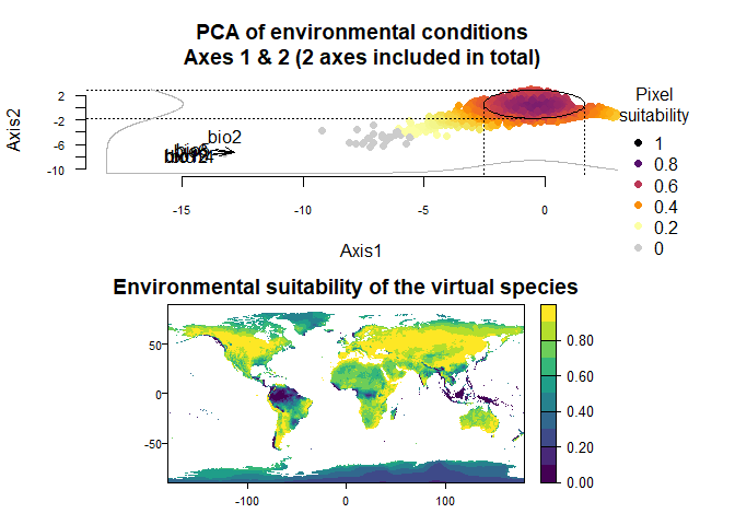
plotResponse(wide.species)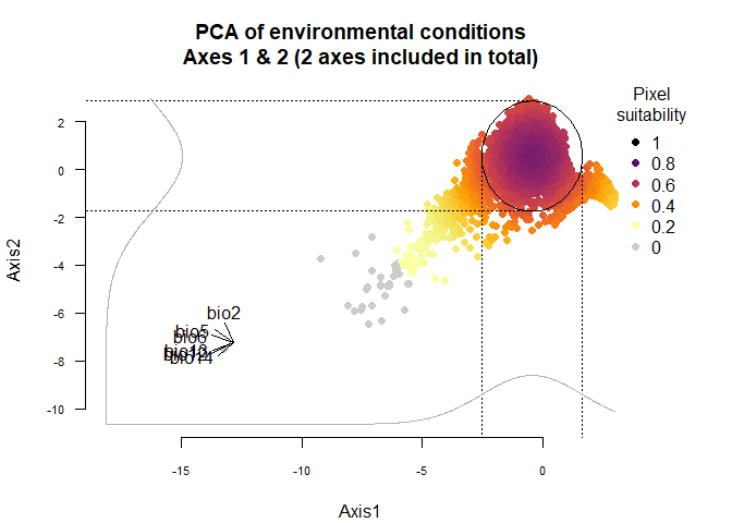
plot(wide.species)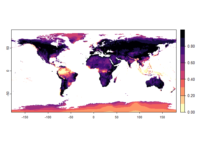
- You can define by yourself the mean and standard deviations of the
Gaussian responses. To do this, use arguments
meansandsdsas in the following example.
Using the figure above, we know that the first axis is driven by precipitation variables, and the second one by temperature variables. To define a species living in colder and wetter environments, we will move the means of Gaussian responses to the right of the first axis (e.g., a mean of 0 or above) and to the top of the second axis (e.g., a mean of 1 or above). In addition, if we want our species to be stenotopic (narrow niche breadth), we will also define lower standard deviations (e.g., standard deviations of 0.25). The correct input will be :means = c(0, 1)(a mean of 0 for the first axis and 1 for the second) andsds = c(0.25, 0.5)(standard deviations of 0.25 for axes 1 and 2):
my.custom.species <- generateSpFromPCA(raster.stack = my.stack,
                                       sample.points = TRUE,
                                       nb.points = 5000,
                                       means = c(0, 1), sds = c(0.5, 0.5))
## - Perfoming the pca## - Defining the response of the species along PCA axes## - You have provided standard deviations, so argument niche.breadth will be ignored.## - Calculating suitability values## The final environmental suitability was rescaled between 0 and 1.
## To disable, set argument rescale = FALSE## Argument rescale was not specified, so it was automatically defined to TRUE. Verify that this is what you want.## No default value was defined for rescale.each.response, setting rescale.each.response = TRUE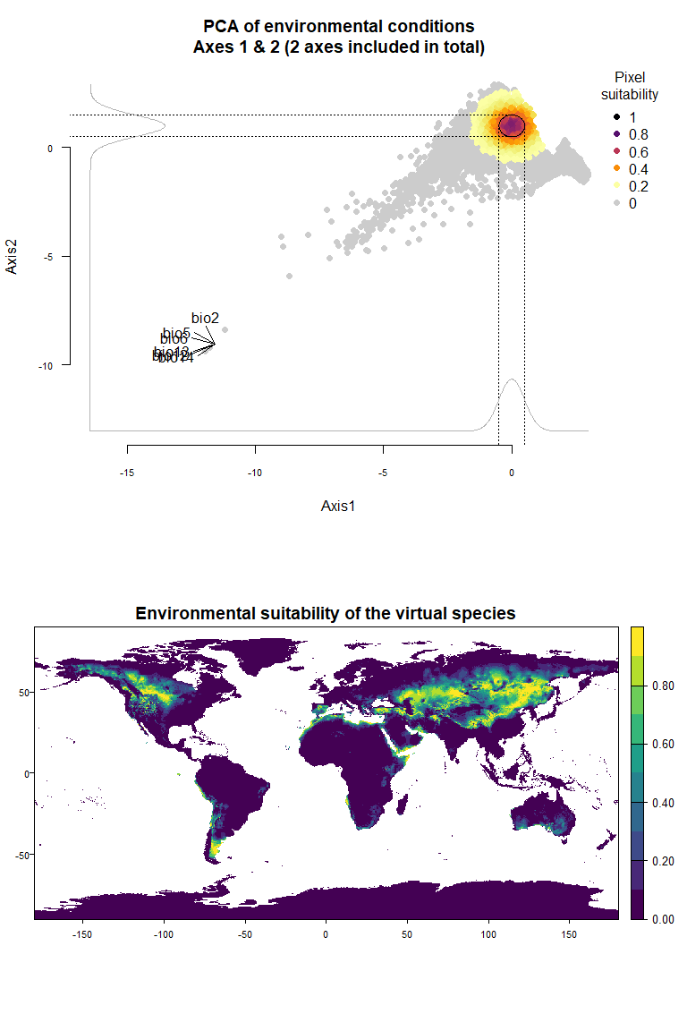
plotResponse(my.custom.species)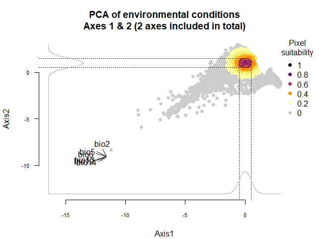
plot(my.custom.species)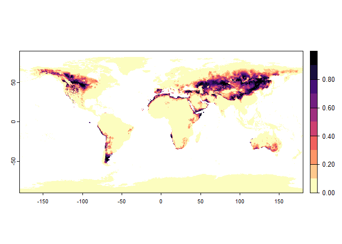
3.2.2. Choosing axes
You can choose the axes generated in the PCA by specifying the axes included in the PCA:
my.custom.species <- generateSpFromPCA(raster.stack = my.stack,
                                       axes = c(1, 3, 5))
## Reading raster values. If it fails for very large rasters, use arguments 'sample.points = TRUE' and define a number of points to sample with 'nb.point'.## - Perfoming the pca## - Defining the response of the species along PCA axes## - Calculating suitability values## The final environmental suitability was rescaled between 0 and 1.
## To disable, set argument rescale = FALSE## Argument rescale was not specified, so it was automatically defined to TRUE. Verify that this is what you want.## No default value was defined for rescale.each.response, setting rescale.each.response = TRUE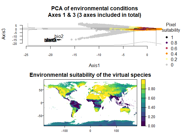
You can see slect which axes you want to see in
plotResponse:
plotResponse(my.custom.species,
             axes = c(1, 5))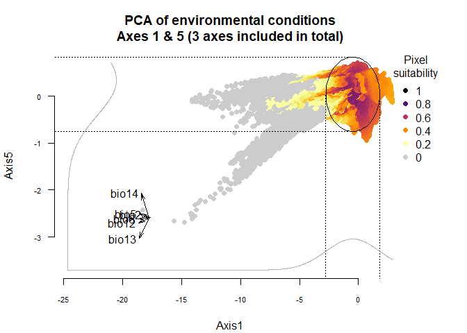
plotResponse(my.custom.species,
             axes = c(3, 5))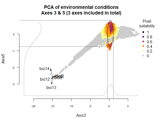
3.2.3. Rescaling of the final environmental suitability
The final rescaling is performed for the same reasons as in
generateSpFromFun. It should not be disabled unless you
have very precise reasons to do it. The argument rescale
controls this rescaling (TRUE by default).
3.2.4. Using a custom PCA
It is possible, if you need, to use your own PCA. In that case, make
sure that the PCA was performed with the function dudi.pca
of the package ade4.
You also need to perform the PCA on the same variables as in your
SpatRaster, entered in the exact same
order.
One reason to use a custom PCA could be that you have a struggling
computer, which requires to generate a PCA from a very reduced subset of
your environmental stack (e.g.,
generateSpFromPCA(my.stack, sample.points = TRUE, nb.points = 250)).
In such a case, the PCA may vary substantially among runs, precluding
any tentative to finely customise the responses to axes. In this case,
it is easy to extract the PCA from a previous run, and use it in the
next run(s):
my.first.run <- generateSpFromPCA(raster.stack = my.stack,
                                  sample.points = TRUE,
                                  nb.points = 250)
## - Perfoming the pca## - Defining the response of the species along PCA axes## - Calculating suitability values## The final environmental suitability was rescaled between 0 and 1.
## To disable, set argument rescale = FALSE## Argument rescale was not specified, so it was automatically defined to TRUE. Verify that this is what you want.## No default value was defined for rescale.each.response, setting rescale.each.response = TRUE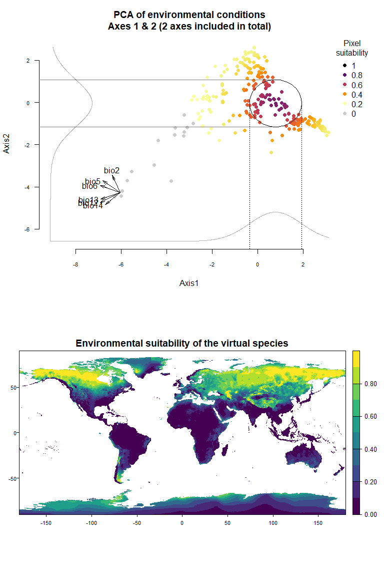
# You can access the PCA with the following command
my.pca <- my.first.run$details$pca

# And then provide it to your second run
my.second.run <- generateSpFromPCA(raster.stack = my.stack,
                                   pca = my.pca)
## Reading raster values. If it fails for very large rasters, use arguments 'sample.points = TRUE' and define a number of points to sample with 'nb.point'.## - Defining the response of the species along PCA axes## - Calculating suitability values## The final environmental suitability was rescaled between 0 and 1.
## To disable, set argument rescale = FALSE## Argument rescale was not specified, so it was automatically defined to TRUE. Verify that this is what you want.## No default value was defined for rescale.each.response, setting rescale.each.response = TRUE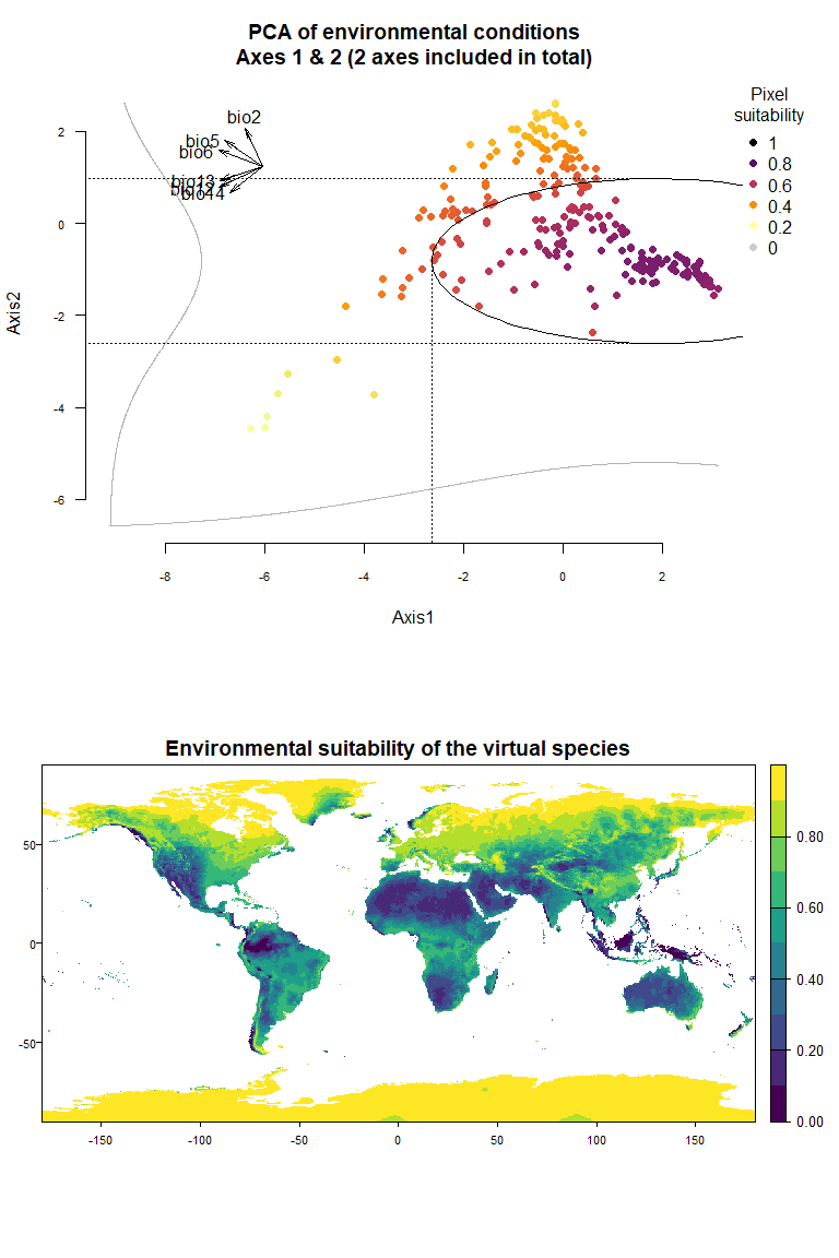
3.2.5. Transferring niches between environmental datasets (e.g., climate change studies)
If you are using virtual species in cases of climate change, you need to keep the virtual niche as it was generated on current data and project it entirely on future data. To do so, you have to use the PCA and responses to PCA axes that were generated on current data, and project them on future data.
Let’s start by generating a virtual species in current conditions:
vs1.current <- generateSpFromPCA(raster.stack = my.stack,
                                 means = c(0, 0), sds = c(1, 1))
## Reading raster values. If it fails for very large rasters, use arguments 'sample.points = TRUE' and define a number of points to sample with 'nb.point'.## - Perfoming the pca## - Defining the response of the species along PCA axes## - You have provided standard deviations, so argument niche.breadth will be ignored.## - Calculating suitability values## The final environmental suitability was rescaled between 0 and 1.
## To disable, set argument rescale = FALSE## Argument rescale was not specified, so it was automatically defined to TRUE. Verify that this is what you want.## No default value was defined for rescale.each.response, setting rescale.each.response = TRUE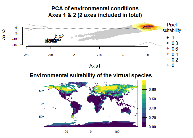
Then, we will project this virtual species onto future conditions:
# Let's get future projections from the CMIP6, SSP scenario 5-8.5, year 2050, model IPSL-CM6A-LR
future.stack <- cmip6_world("IPSL-CM6A-LR", var = "bioc", res = 10,
                            ssp = 585, time = "2041-2060",
                            path = tempdir())
names(future.stack) <- paste0("bio", 1:19)
future.stack <- future.stack[[c("bio2", "bio5", "bio6", "bio12", "bio13", "bio14")]]

# Now let's project our virtual species into the future
vs1.future <- generateSpFromPCA(raster.stack = future.stack,
                                 pca = vs1.current$details$pca,
                                 means = vs1.current$details$means,
                                 sds = vs1.current$details$sds)
## Reading raster values. If it fails for very large rasters, use arguments 'sample.points = TRUE' and define a number of points to sample with 'nb.point'.## - Defining the response of the species along PCA axes## - You have provided standard deviations, so argument niche.breadth will be ignored.## - Calculating suitability values## The final environmental suitability was rescaled between 0 and 1.
## To disable, set argument rescale = FALSE## Argument rescale was not specified, so it was automatically defined to TRUE. Verify that this is what you want.## No default value was defined for rescale.each.response, setting rescale.each.response = TRUE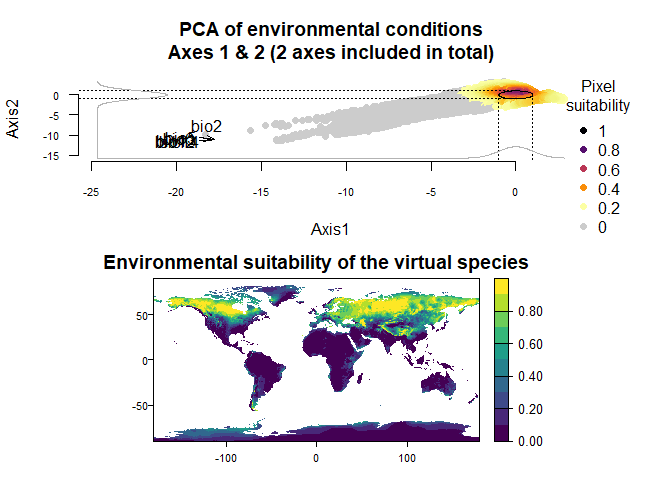
You can see how the species range will shift northward. Will your sdms correctly predict it? ;)
-----------------
Do not hesitate if you have a question, find a bug, or would like to add a feature in virtualspecies: mail me!