7. Sampling occurrences
7.1. Basic usage
If you generated virtual species distributions with this package,
there is a good chance that your objective is to test a particular
modelling protocol or technique. Hence, there is one last step for you
to perform: the sampling of species occurrences. This can be done with
the function sampleOccurrences, with which you can sample
either “presence-absence” or “presence only” occurrence data. The
function sampleOccurrences also provides the possibility to
introduce a number of sampling biases, such as uneven spatial sampling
intensity, probability of detection, and probability of error.
Let’s see an example in practice, using the same tropical species we generated in the beginning of this tutorial:
library(virtualspecies)## Le chargement a nécessité le package : terra## terra 1.7.46## The legacy packages maptools, rgdal, and rgeos, underpinning the sp package,
## which was just loaded, will retire in October 2023.
## Please refer to R-spatial evolution reports for details, especially
## https://r-spatial.org/r/2023/05/15/evolution4.html.
## It may be desirable to make the sf package available;
## package maintainers should consider adding sf to Suggests:.
## The sp package is now running under evolution status 2
## (status 2 uses the sf package in place of rgdal)library(geodata)
# Worldclim data
worldclim <- worldclim_global(var = "bio", res = 10,
path = tempdir())
names(worldclim) <- paste0("bio", 1:19)
# Formatting of the response functions
my.parameters <- formatFunctions(bio1 = c(fun = 'dnorm', mean = 25, sd = 5),
bio12 = c(fun = 'dnorm', mean = 4000, sd = 2000))
# Generation of the virtual species
my.first.species <- generateSpFromFun(raster.stack = worldclim[[c("bio1", "bio12")]],
parameters = my.parameters)## Generating virtual species environmental suitability...## - The response to each variable was rescaled between 0 and 1. To
## disable, set argument rescale.each.response = FALSE## - The final environmental suitability was rescaled between 0 and 1. To disable, set argument rescale = FALSE# Conversion to presence-absence
my.first.species <- convertToPA(my.first.species,
beta = 0.7, plot = FALSE)## --- Determing species.prevalence automatically according to alpha and beta## Logistic conversion finished:
##
## - beta = 0.7
## - alpha = -0.05
## - species prevalence =0.0244971555083639# Sampling of 'presence only' occurrences
presence.points <- sampleOccurrences(my.first.species,
n = 30, # The number of points to sample
type = "presence only")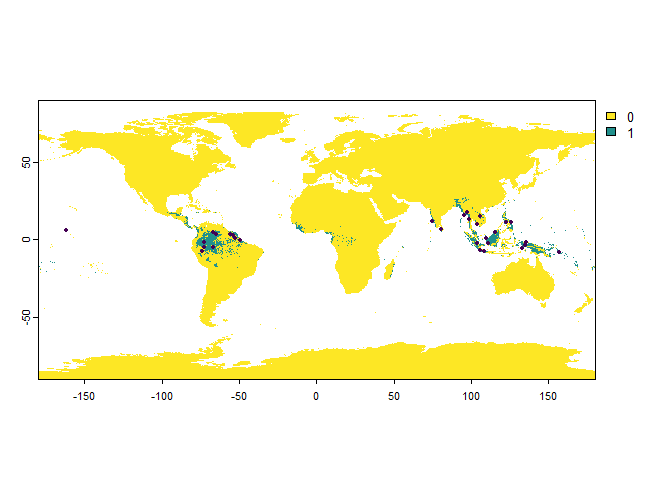
We can see that a map was plotted, with the sampled presence points illustrated with black dots.
Now let’s see how our object presence.points looks
like:
presence.points## Occurrence points sampled from a virtual species
##
## - Type: presence only
## - Number of points: 30
## - No sampling bias
## - Detection probability:
## .Probability: 1
## .Corrected by suitability: FALSE
## - Probability of identification error (false positive): 0
## - Multiple samples can occur in a single cell: No
##
## First 10 lines:
## x y Real Observed
## 1088748 -162.08333 5.916667 1 1
## 1237397 132.75000 -5.416667 1 1
## 1231880 -66.75000 -5.083333 1 1
## 1121785 -55.91667 3.416667 1 1
## 1169344 -49.41667 -0.250000 1 1
## 1215812 135.25000 -3.750000 1 1
## 1263173 108.75000 -7.416667 1 1
## 939106 97.58333 17.583333 1 1
## 1266396 -74.08333 -7.750000 1 1
## 1256676 105.91667 -6.916667 1 1
## ... 20 more lines.This message summarizes us information about the 30 occurrence points we just sampled. Now let’s look at the structure of this object:
str(presence.points)## List of 8
## $ type : chr "presence only"
## $ detection.probability :List of 2
## ..$ detection.probability : num 1
## ..$ correct.by.suitability: logi FALSE
## $ error.probability : num 0
## $ bias : NULL
## $ replacement : logi FALSE
## $ original.distribution.raster:S4 class 'SpatRaster' [package "terra"]
## $ sample.plot :List of 3
## ..$ :Dotted pair list of 24
## ..$ : raw [1:35992] 00 00 00 00 ...
## .. ..- attr(*, "pkgName")= chr "graphics"
## ..$ :List of 2
## .. ..- attr(*, "pkgName")= chr "grid"
## ..- attr(*, "engineVersion")= int 16
## ..- attr(*, "pid")= int 31592
## ..- attr(*, "Rversion")=Classes 'R_system_version', 'package_version', 'numeric_version' hidden list of 1
## ..- attr(*, "load")= chr(0)
## ..- attr(*, "attach")= chr(0)
## ..- attr(*, "class")= chr "recordedplot"
## $ sample.points :'data.frame': 30 obs. of 4 variables:
## ..$ x : num [1:30] -162.1 132.8 -66.8 -55.9 -49.4 ...
## ..$ y : num [1:30] 5.92 -5.42 -5.08 3.42 -0.25 ...
## ..$ Real : num [1:30] 1 1 1 1 1 1 1 1 1 1 ...
## ..$ Observed: num [1:30] 1 1 1 1 1 1 1 1 1 1 ...
## - attr(*, "RNGkind")= chr [1:3] "Mersenne-Twister" "Inversion" "Rejection"
## - attr(*, "seed")= int [1:626] 10403 288 -962552501 -84035233 1038343804 1488043481 889822882 1185920310 -301917002 -1257285662 ...
## - attr(*, "class")= chr [1:2] "VSSampledPoints" "list"This is a list containing eight elements:
type: the type of occurrence sampled (presence absence or presence-only)detection.probability: the detection probability of our virtual specieserror.probability: the probability of an erroneous detection of our virtual speciesbias: if you introduced a sampling bias, this part will contain the appropriate inforeplacement: a logical indicating if you allowed multiple samples in the same cellsoriginal.distribution.raster: the raster from which occurrences were sampledsample.plot: contains the graphical representation of your samples, so it can be called latersampled.points: a data frame containing the sampled points
It also says to us that there are several attributes stored, such as
the information about the randomisation process (RNGkind
and seed). You can use these attributes later to reproduce
exactly a previous sampling.
Now, we can specifically access the data frame of sampled points:
presence.points$sample.points## x y Real Observed
## 1088748 -162.08333 5.9166667 1 1
## 1237397 132.75000 -5.4166667 1 1
## 1231880 -66.75000 -5.0833333 1 1
## 1121785 -55.91667 3.4166667 1 1
## 1169344 -49.41667 -0.2500000 1 1
## 1215812 135.25000 -3.7500000 1 1
## 1263173 108.75000 -7.4166667 1 1
## 939106 97.58333 17.5833333 1 1
## 1266396 -74.08333 -7.7500000 1 1
## 1256676 105.91667 -6.9166667 1 1
## 1036344 103.91667 10.0833333 1 1
## 1079403 80.41667 6.7500000 1 1
## 1123891 -64.91667 3.2500000 1 1
## 1274263 157.08333 -8.2500000 1 1
## 1128276 -54.08333 2.9166667 1 1
## 1008091 75.08333 12.2500000 1 1
## 1190806 -72.41667 -1.9166667 1 1
## 1227526 -72.41667 -4.7500000 1 1
## 1185573 135.41667 -1.4166667 1 1
## 1194022 103.58333 -2.0833333 1 1
## 1017015 122.41667 11.5833333 1 1
## 1106601 -66.58333 4.5833333 1 1
## 967236 105.91667 15.4166667 1 1
## 993113 98.75000 13.4166667 1 1
## 1198388 111.25000 -2.4166667 1 1
## 1107692 115.25000 4.5833333 1 1
## 1150857 109.41667 1.2500000 1 1
## 1154207 -52.25000 0.9166667 1 1
## 962853 95.41667 15.7500000 1 1
## 1023515 125.75000 11.0833333 1 1The data frame has four colums: the pixel coordinates x
and y, the real presence/absence (1/0) of the species in
the sampled pixel Real, and the result of the sampling
Observed (1 = presence, 0 = absence, NA = no information).
The columns Real and Observed differ only if
you have specified a detection probability and/or an error
probability.
Now, let’s sample the other type of occurrence data: presence-absence.
# Sampling of 'presence-absence' occurrences
PA.points <- sampleOccurrences(my.first.species,
                               n = 300,
                               type = "presence-absence")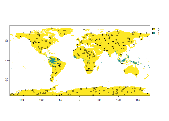
PA.points## Occurrence points sampled from a virtual species
##
## - Type: presence-absence
## - Number of points: 300
## - No sampling bias
## - Detection probability:
## .Probability: 1
## .Corrected by suitability: FALSE
## - Probability of identification error (false positive): 0
## - Sample prevalence:
## .True:0.01
## .Observed:0.01
## - Multiple samples can occur in a single cell: No
##
## First 10 lines:
## x y Real Observed
## 171413 -51.25000 76.75000 0 0
## 479386 157.58333 53.08333 0 0
## 791057 -97.25000 28.91667 0 0
## 2298665 -109.25000 -87.41667 0 0
## 2083546 37.58333 -70.75000 0 0
## 599737 56.08333 43.75000 0 0
## 2043008 121.25000 -67.58333 0 0
## 712122 66.91667 35.08333 0 0
## 773755 -100.91667 30.25000 0 0
## 554845 134.08333 47.25000 0 0
## ... 290 more lines.You can see that the points are sampled randomly throughout the whole
raster. However, we may have only a few or even no presence points at
all because the samples are purely random at the moment. We can define
the number of presences and the number of absences by using the
parameter sample.prevalence.
You may be interested in extracting the true probability of
occurrence at each sampled point, to compare with your SDM results. To
do this, use argument extract.probability:
# Sampling of 'presence-absence' occurrences
PA.points <- sampleOccurrences(my.first.species,
                               n = 30,
                               type = "presence-absence",
                               extract.probability = TRUE,
                               plot = FALSE)
PA.points
## Occurrence points sampled from a virtual species
##
## - Type: presence-absence
## - Number of points: 30
## - No sampling bias
## - Detection probability:
## .Probability: 1
## .Corrected by suitability: FALSE
## - Probability of identification error (false positive): 0
## - Sample prevalence:
## .True:0
## .Observed:0
## - Multiple samples can occur in a single cell: No
##
## First 10 lines:
## x y Real Observed true.probability
## 670998 52.91667 38.250000 0 0 1.658934e-06
## 894718 -100.41667 20.916667 0 0 2.151494e-06
## 2146264 50.58333 -75.583333 0 0 8.315280e-07
## 1272000 139.91667 -8.083333 0 0 9.830516e-03
## 2149559 -120.25000 -75.916667 0 0 8.315280e-07
## 274191 158.41667 68.916667 0 0 8.315280e-07
## 2286879 86.41667 -86.416667 0 0 8.315280e-07
## 558885 87.41667 46.916667 0 0 8.333703e-07
## 730586 -95.75000 33.583333 0 0 6.658379e-06
## 2088575 155.75000 -71.083333 0 0 8.315280e-07
## ... 20 more lines.In the next section you will see how to limit the sampling to a region in particular, and after that, how to introduce a bias in the sampling procedure.
7.2. Delimiting a sampling area
There are three main possibilities to delimit the sampling areas :
- Specifying the region(s) of the world (country, continent, region
- Provide a polygon (of type
SpatialPolygonsorSpatialPolygonsDataFrameof packagesp) - Provide an
extentobject (a rectangular area, from the packageraster)
7.2.1. Specifying the region(s) of the world
You can specify any combination of countries, continents and regions
of the world to restrict your sampling area, using the argument
sampling.area. For example:
# Sampling of 'presence-absence' occurrences
PA.points <- sampleOccurrences(my.first.species,
                               n = 30,
                               type = "presence-absence",
                               sampling.area = c("South America", "Mexico"))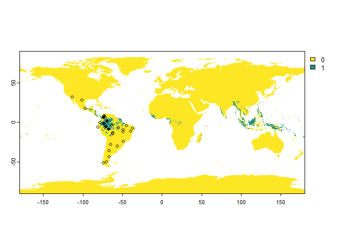
The only restriction is to provide the correct names and to have the
package rnaturalearth installed.
The correct region names are: “Africa”, “Antarctica”, “Asia”, “Oceania”, “Europe”, “Americas”
The correct continent names are: “Africa”, “Antarctica”, “Asia”, “Europe”, “North America”, “Oceania”, “South America”
And you can consult the correct names with the following commands:
# Country names
 unique(rnaturalearth::ne_countries(returnclass ='sf')$sovereignt)
## [1] "Fiji" "United Republic of Tanzania"
## [3] "Western Sahara" "Canada"
## [5] "United States of America" "Kazakhstan"
## [7] "Uzbekistan" "Papua New Guinea"
## [9] "Indonesia" "Argentina"
## [11] "Chile" "Democratic Republic of the Congo"
## [13] "Somalia" "Kenya"
## [15] "Sudan" "Chad"
## [17] "Haiti" "Dominican Republic"
## [19] "Russia" "The Bahamas"
## [21] "United Kingdom" "Norway"
## [23] "Denmark" "France"
## [25] "East Timor" "South Africa"
## [27] "Lesotho" "Mexico"
## [29] "Uruguay" "Brazil"
## [31] "Bolivia" "Peru"
## [33] "Colombia" "Panama"
## [35] "Costa Rica" "Nicaragua"
## [37] "Honduras" "El Salvador"
## [39] "Guatemala" "Belize"
## [41] "Venezuela" "Guyana"
## [43] "Suriname" "Ecuador"
## [45] "Jamaica" "Cuba"
## [47] "Zimbabwe" "Botswana"
## [49] "Namibia" "Senegal"
## [51] "Mali" "Mauritania"
## [53] "Benin" "Niger"
## [55] "Nigeria" "Cameroon"
## [57] "Togo" "Ghana"
## [59] "Ivory Coast" "Guinea"
## [61] "Guinea-Bissau" "Liberia"
## [63] "Sierra Leone" "Burkina Faso"
## [65] "Central African Republic" "Republic of the Congo"
## [67] "Gabon" "Equatorial Guinea"
## [69] "Zambia" "Malawi"
## [71] "Mozambique" "eSwatini"
## [73] "Angola" "Burundi"
## [75] "Israel" "Lebanon"
## [77] "Madagascar" "Gambia"
## [79] "Tunisia" "Algeria"
## [81] "Jordan" "United Arab Emirates"
## [83] "Qatar" "Kuwait"
## [85] "Iraq" "Oman"
## [87] "Vanuatu" "Cambodia"
## [89] "Thailand" "Laos"
## [91] "Myanmar" "Vietnam"
## [93] "North Korea" "South Korea"
## [95] "Mongolia" "India"
## [97] "Bangladesh" "Bhutan"
## [99] "Nepal" "Pakistan"
## [101] "Afghanistan" "Tajikistan"
## [103] "Kyrgyzstan" "Turkmenistan"
## [105] "Iran" "Syria"
## [107] "Armenia" "Sweden"
## [109] "Belarus" "Ukraine"
## [111] "Poland" "Austria"
## [113] "Hungary" "Moldova"
## [115] "Romania" "Lithuania"
## [117] "Latvia" "Estonia"
## [119] "Germany" "Bulgaria"
## [121] "Greece" "Turkey"
## [123] "Albania" "Croatia"
## [125] "Switzerland" "Luxembourg"
## [127] "Belgium" "Netherlands"
## [129] "Portugal" "Spain"
## [131] "Ireland" "Solomon Islands"
## [133] "New Zealand" "Australia"
## [135] "Sri Lanka" "China"
## [137] "Taiwan" "Italy"
## [139] "Iceland" "Azerbaijan"
## [141] "Georgia" "Philippines"
## [143] "Malaysia" "Brunei"
## [145] "Slovenia" "Finland"
## [147] "Slovakia" "Czechia"
## [149] "Eritrea" "Japan"
## [151] "Paraguay" "Yemen"
## [153] "Saudi Arabia" "Antarctica"
## [155] "Northern Cyprus" "Cyprus"
## [157] "Morocco" "Egypt"
## [159] "Libya" "Ethiopia"
## [161] "Djibouti" "Somaliland"
## [163] "Uganda" "Rwanda"
## [165] "Bosnia and Herzegovina" "North Macedonia"
## [167] "Republic of Serbia" "Montenegro"
## [169] "Kosovo" "Trinidad and Tobago"
## [171] "South Sudan"7.2.2. Providing a polygon
In this case you have to import in R your own polygon, using commands
of packages sf or terra.
We will use here an example of a terra object which we
can downloaded straight into R using the R package geodata.
Since our species is a tropical species, let’s assume we are working in
Brazil only. Remember that this is an example, and that you can import
your own polygons into R.
First, let’s download our polygon:
brazil <- gadm(country = "BRA", level = 0, path = tempdir())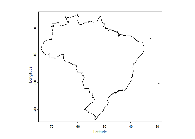
Now, to limit the sampling area to our polygon, we simply provide it
to the argument sampling.area of the function
sampleOccurrences():
PA.points <- sampleOccurrences(my.first.species,
                               n = 30,
                               type = "presence-absence",
                               sampling.area = brazil)
PA.points## Occurrence points sampled from a virtual species
##
## - Type: presence-absence
## - Number of points: 30
## - No sampling bias
## - Detection probability:
## .Probability: 1
## .Corrected by suitability: FALSE
## - Probability of identification error (false positive): 0
## - Sample prevalence:
## .True:0.133333333333333
## .Observed:0.133333333333333
## - Multiple samples can occur in a single cell: No
##
## First 10 lines:
## x y Real Observed
## 1432910 -41.75000 -20.5833333 0 0
## 1456600 -53.41667 -22.4166667 0 0
## 1435026 -49.08333 -20.7500000 0 0
## 1242853 -37.91667 -5.9166667 0 0
## 1221202 -46.41667 -4.2500000 0 0
## 1346456 -50.75000 -13.9166667 0 0
## 1149845 -59.25000 1.2500000 1 1
## 1277399 -40.25000 -8.5833333 0 0
## 1160682 -53.08333 0.4166667 0 0
## 1203856 -57.41667 -2.9166667 1 1
## ... 20 more lines.It worked!
However, the plot is not very convenient because it kept the scale of our input raster, so we may be interested in manually restricting the plot region to Brasil:
# First we get our data frame of occurrence points
occ <- PA.points$sample.points

plot(my.first.species$pa.raster,
     xlim = c(-80, -30),
     ylim = c(-35, 10))
plot(brazil, add = TRUE)
points(occ[occ$Observed == 1, c("x", "y")], pch = 16, cex = .8)
points(occ[occ$Observed == 0, c("x", "y")], pch = 1, cex = .8)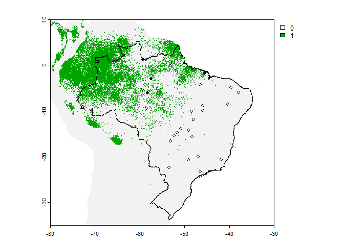
7.2.3. Providing an extent object
An extent object is a rectangular area defined by four coordinates
xmin/xmax/ymin/ymax. You can easily create an extent object using the
command extent, of the package raster:
my.extent <- ext(-80, -30, -35, 10)
PA.points <- sampleOccurrences(my.first.species,
                               n = 30,
                               type = "presence-absence",
                               sampling.area = my.extent)
plot(my.extent, add = TRUE)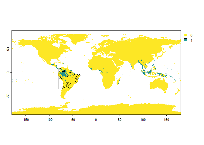
7.2.4 Draw an extent or a polygon to sample
You can draw a polygon manually with terra and feed it
to sampleOccurrences, try it yourself (press ‘escape’ when
finished):
plot(my.first.species$pa.raster)
my.polygon <- terra::draw(x = "polygon")
7.3. Introducing a sampling bias
7.3.1.Detection probability
Detection probability has been shown to be influential on SDM
performance. Hence, you might be interested in generating species with
varying degrees of detection probability. This can be done easily, using
the argument detection.probability, ranging from 0 (species
cannot be detected) to 1 (species is always detected):
# Let's try to find samples of a very cryptic species
PA.points <- sampleOccurrences(my.first.species,
                               sampling.area = "Brazil",
                               n = 50,
                               type = "presence-absence",
                               detection.probability = 0.3)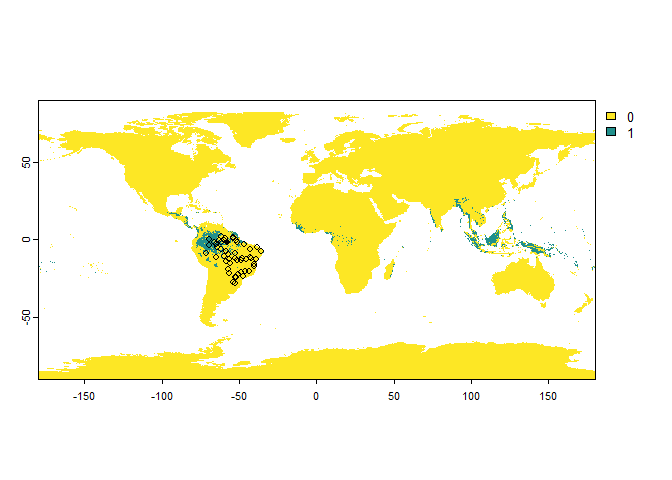
PA.points## Occurrence points sampled from a virtual species
##
## - Type: presence-absence
## - Number of points: 50
## - No sampling bias
## - Detection probability:
## .Probability: 0.3
## .Corrected by suitability: FALSE
## - Probability of identification error (false positive): 0
## - Sample prevalence:
## .True:0.12
## .Observed:0.02
## - Multiple samples can occur in a single cell: No
##
## First 10 lines:
## x y Real Observed
## 1326981 -56.58333 -12.4166667 1 0
## 1309652 -64.75000 -11.0833333 0 0
## 1156359 -53.58333 0.7500000 0 0
## 1171444 -59.41667 -0.4166667 0 0
## 1247144 -42.75000 -6.2500000 0 0
## 1184414 -57.75000 -1.4166667 1 1
## 1139030 -61.75000 2.0833333 0 0
## 1290259 -56.91667 -9.5833333 0 0
## 1327085 -39.25000 -12.4166667 0 0
## 1374598 -40.41667 -16.0833333 0 0
## ... 40 more lines.You can see that some points sampled in its distribution range are classified as “absences”.
If you use this argument when sampling ‘presence only’ occurrences, then this will result in a lower number of sampled points than asked:
PO.points <- sampleOccurrences(my.first.species,
                               sampling.area = "Brazil",
                               n = 50,
                               type = "presence only",
                               detection.probability = 0.3)
PO.points## Occurrence points sampled from a virtual species
##
## - Type: presence only
## - Number of points: 50
## - No sampling bias
## - Detection probability:
## .Probability: 0.3
## .Corrected by suitability: FALSE
## - Probability of identification error (false positive): 0
## - Multiple samples can occur in a single cell: No
##
## First 10 lines:
## x y Real Observed
## 1247014 -64.41667 -6.250000 1 NA
## 1257867 -55.58333 -7.083333 1 NA
## 1218920 -66.75000 -4.083333 1 1
## 1184404 -59.41667 -1.416667 1 NA
## 1186618 -50.41667 -1.583333 1 1
## 1227529 -71.91667 -4.750000 1 NA
## 1186570 -58.41667 -1.583333 1 NA
## 1253482 -66.41667 -6.750000 1 NA
## 1156296 -64.08333 0.750000 1 1
## 1236182 -69.75000 -5.416667 1 NA
## ... 40 more lines.In this case, we see that out of all the possible sampling points, only a fraction are sampled as presence points.
7.3.2. Detection probability as a function of environmental suitability
You can further complexify the detection probability by making it dependent on the environmental suitability. In this case, cells will be weighted by the environmental suitability: less suitable cells will have a lesser chance of detecting the species. This can be seen as an impact on the population size: a higher environmental suitability increases the population size, and thus the detection probability. How does this work in practice?
The initial probability of detection (\(P_{di}\)) is multiplied by the environmental suitability (\(S\)) to obtain the final probability of detection (\(P_d\)):
\[P_d = P_{di} \times S\]
Hence, if our species has a probability of detection of 0.5, the final probability of detection will be:
- 0.5 if the cell has an environmental suitability of 1
- 0.25 if the cell has an environmental suitability of 0.5
Of course, no occurrence points will be detected outside the distribution range, regardless of their environmental suitability.
You can also keep the detection probability to 1, and set
correct.by.suitability = TRUE. In that case, the detection
probability will be equal to the environmental suitability. This can be
seen as a species whose detection probability is strictly dependent on
its population size, which in turn is strictly dependent on the
environmental suitability.
An example in practice:
PA.points <- sampleOccurrences(my.first.species,
                               sampling.area = "Brazil",
                               n = 100,
                               type = "presence-absence",
                               detection.probability = 1,
                               correct.by.suitability = TRUE,
                               plot = FALSE)

# Below is a custom plot to show the sampled point above the map of environmental suitability
occ <- PA.points$sample.points

plot(my.first.species$suitab.raster,
     xlim = c(-80, -20),
     ylim = c(-35, 5))
# plot(brasil, add = TRUE)
points(occ[occ$Observed == 1, c("x", "y")], pch = 16, cex = .8)
points(occ[occ$Observed == 0, c("x", "y")], pch = 1, cex = .8)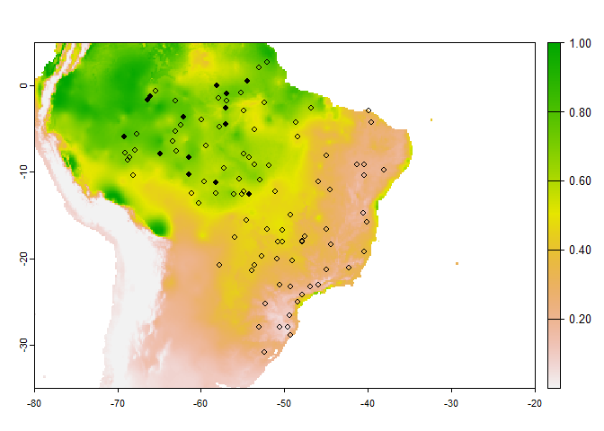
7.3.3. Error probability
You can also introduce an error probability, which is a probability
of finding the species where it is absent. This is straightforward with
the argument error.probability:
PA.points <- sampleOccurrences(my.first.species,
                               sampling.area = "Brazil",
                               n = 20,
                               type = "presence-absence",
                               error.probability = 0.3)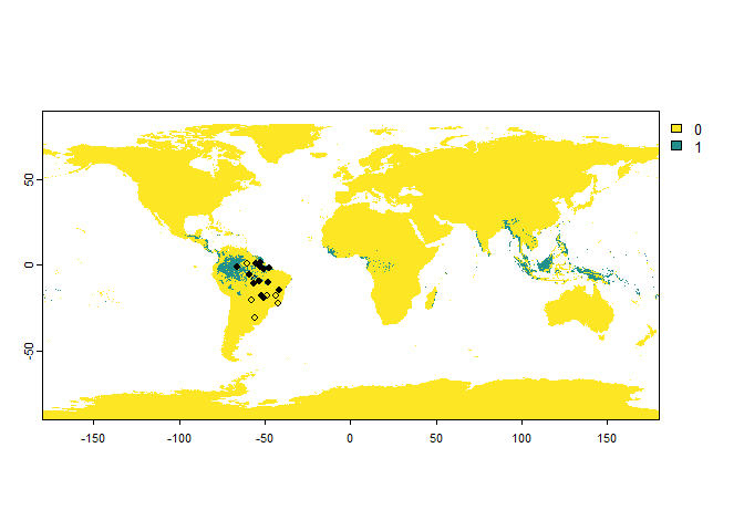
PA.points## Occurrence points sampled from a virtual species
##
## - Type: presence-absence
## - Number of points: 20
## - No sampling bias
## - Detection probability:
## .Probability: 1
## .Corrected by suitability: FALSE
## - Probability of identification error (false positive): 0.3
## - Sample prevalence:
## .True:0.3
## .Observed:0.65
## - Multiple samples can occur in a single cell: No
##
## First 10 lines:
## x y Real Observed
## 1147727 -52.25000 1.416667 1 1
## 1188797 -47.25000 -1.750000 1 1
## 1560265 -55.91667 -30.416667 0 0
## 1350831 -41.58333 -14.250000 0 1
## 1303221 -56.58333 -10.583333 0 1
## 1197415 -50.91667 -2.416667 1 1
## 1394019 -43.58333 -17.583333 0 0
## 1290282 -53.08333 -9.583333 1 1
## 1413416 -50.75000 -19.083333 0 1
## 1396147 -48.91667 -17.750000 0 0
## ... 10 more lines.One important remark with the error probability:
There is an interaction between the detection probability and the error probability: in a cell where the species is present, but not detected, a presence can still be attributed because of an error. See the following (extreme) example, for a species with a low detection probability and high error probability:
PA.points <- sampleOccurrences(my.first.species,
                               sampling.area = "Brazil",
                               n = 20,
                               type = "presence-absence",
                               detection.probability = 0.2,
                               error.probability = 0.8)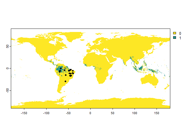
PA.points## Occurrence points sampled from a virtual species
##
## - Type: presence-absence
## - Number of points: 20
## - No sampling bias
## - Detection probability:
## .Probability: 0.2
## .Corrected by suitability: FALSE
## - Probability of identification error (false positive): 0.8
## - Sample prevalence:
## .True:0.15
## .Observed:0.9
## - Multiple samples can occur in a single cell: No
##
## First 10 lines:
## x y Real Observed
## 1378884 -46.08333 -16.416667 0 1
## 1234154 -47.75000 -5.250000 0 1
## 1383218 -43.75000 -16.750000 0 1
## 1234201 -39.91667 -5.250000 0 1
## 1305484 -39.41667 -10.750000 0 1
## 1156333 -57.91667 0.750000 0 0
## 1212569 -45.25000 -3.583333 0 1
## 1320571 -44.91667 -11.916667 0 1
## 1314075 -47.58333 -11.416667 0 1
## 1385367 -45.58333 -16.916667 0 1
## ... 10 more lines.7.3.4. Uneven sampling intensity
The sampleOccurrences also allows you to introduce a
sampling bias such as uneven sampling intensity in space. How does it
works?
You will have to define a region in which the sampling is biased,
with arguments bias and area. In this region,
the sampling will be biased by a strength equal to the argument
bias.strength. If bias.strength is equal to 50
for example, then the sampling will be 50 times more intense in the
chosen area. If bias.strengthis below 1, then the sampling
will be less intense in the biased area than elsewhere.
Let’s see an example in practice before we go into the details:
PO.points <- sampleOccurrences(my.first.species,
                               n = 100,
                               bias = "continent",
                               bias.strength = 20,
                               bias.area = "South America")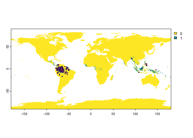
Now that you have grasped how the bias works, let’s see the different possibilities:
- Introducing a bias using country, region or continent names
Set eitherbias = "country",bias = "region"orbias = "continent", and provide tobias.areathe name(s) of the country(-ies), region(s) or continent(s).
PO.points <- sampleOccurrences(my.first.species,
                               n = 100,
                               bias = "country",
                               bias.strength = 20,
                               bias.area = c("Mexico", "Colombia"))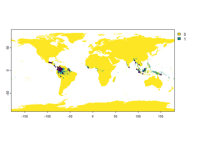
- Using a polygon in which the sampling will be biased
Setbias = "polygon", and provide a polygon (sforterraobject, classessforSpatVector) to the argumentbias.area.
philippines <- rnaturalearth::ne_countries(country = "Philippines",
                                           returnclass = "sf")
PO.points <- sampleOccurrences(my.first.species,
                               n = 100,
                               bias = "polygon",
                               bias.strength = 50,
                               bias.area = philippines)
- Using an extent object
Setbias = "extent", and provide an extent to the argumentbias.area(see section 7.2.3. if you are not familiar with extents). You can also simply setbias = "polygon"(new in version 1.6) orbias = "extent", and click on the map when asked to:
PO.points <- sampleOccurrences(my.first.species,
                               n = 100,
                               bias = "polygon", # also works with "extent"
bias.strength = 50)- Manually defining weights for all the cells
A last option is to manually define the weights with which the sampling will be biased. This may be especially useful when you want to precisely create a sampling bias. To do this, setbias = "manual", and provide a raster of weights to the argumentweights.
To clear things up, we will see an example together:
# First, we create a raster of weights
# As an arbitrary example, we will use the area of each cell as a weight:
# larger cells have more chance of being sampled
weight.raster <- cellSize(worldclim)

plot(weight.raster)
# Add continents
plot(rnaturalearth::ne_coastline(returnclass = "sf")[1], add = TRUE)
Now, let’s weight our samples using this raster:
PO.points <- sampleOccurrences(my.first.species,
                               n = 100,
                               bias = "manual",
                               weights = weight.raster)
Of course, the changes are not visible, because our species occurs mainly in pixels of relatively similar areas. Nevertheless, this example should be useful if you want to create a manual sampling bias later on.
7.3.5. Sampling multiple records in the same cells
In real datasets such as Museum datasets, it is frequent to have multiple records in the same cells. To mimic such datasets, it is possible to allow the function to sample repeatedly in the same cells:
PO.points <- sampleOccurrences(my.first.species,
                               n = 1000,
                               replacement = TRUE,
                               plot = FALSE)

# Number of duplicated records:
length(which(duplicated(PO.points$sample.points[, c("x", "y")])))
## [1] 207.4. Defining the sample prevalence
The sample prevalence is the proportion of samples in which the species has been found. It is therefore different from the species prevalence which was mentionned earlier.
You can define the desired sample prevalence when sampling presences
and absences, with the parameter sample.prevalence:
PA.points <- sampleOccurrences(my.first.species,
                               n = 30,
                               type = "presence-absence",
                               sample.prevalence = 0.5)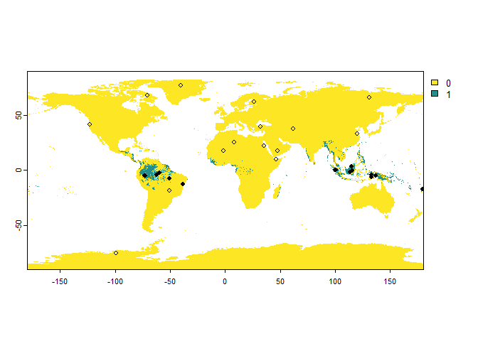
PA.points## Occurrence points sampled from a virtual species
##
## - Type: presence-absence
## - Number of points: 30
## - No sampling bias
## - Detection probability:
## .Probability: 1
## .Corrected by suitability: FALSE
## - Probability of identification error (false positive): 0
## - Sample prevalence:
## .True:0.5
## .Observed:0.5
## - Multiple samples can occur in a single cell: No
##
## First 10 lines:
## x y Real Observed
## 1170333 115.41667 -0.25000000 1 1
## 1220119 133.08333 -4.08333333 1 1
## 1391037 179.41667 -17.25000000 1 1
## 1195202 -59.75000 -2.25000000 1 1
## 1189764 113.91667 -1.75000000 1 1
## 1161599 99.75000 0.41666667 1 1
## 1230943 137.08333 -4.91666667 1 1
## 1260058 -50.41667 -7.25000000 1 1
## 1218947 -62.25000 -4.08333333 1 1
## 1165926 100.91667 0.08333333 1 1
## ... 20 more lines.
-----------------
Do not hesitate if you have a question, find a bug, or would like to add a feature in virtualspecies: mail me!