2. Virtual species defined by response to environmental variables
The first approach to generate a virtual species consists in defining
its response functions to each of the environmental variables contained
in our RasterStack. These responses are then combined to
calculcate the environmental suitability of the virtual species.
The function providing this approach is
generateSpFromFun.
2.1. An introduction example
Before we start using the package, let’s prepare our first simulation of virtual species.
We want to generate a virtual species with two environmental
variables, the annual mean temperature bio1 and annual mean
precipitation bio2. We want to generate a tropical species,
i.e., living in hot and humid environments. We can define bell-shaped
response functions to these two variables, as in the following
figure:
## Le chargement a nécessité le package : terra## terra 1.7.46## The legacy packages maptools, rgdal, and rgeos, underpinning the sp package,
## which was just loaded, will retire in October 2023.
## Please refer to R-spatial evolution reports for details, especially
## https://r-spatial.org/r/2023/05/15/evolution4.html.
## It may be desirable to make the sf package available;
## package maintainers should consider adding sf to Suggests:.
## The sp package is now running under evolution status 2
## (status 2 uses the sf package in place of rgdal)## No default value was defined for rescale.each.response, setting rescale.each.response = TRUE## No default value was defined for rescale.each.response, setting rescale.each.response = TRUE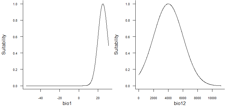
These bell-shaped functions are in fact gaussian distributions functions of the form:
\[ f(x, \mu, \sigma) = \frac{1}{\sigma\sqrt{2\pi}}\, e^{-\frac{(x - \mu)^2}{2 \sigma^2}}\]
If we take the example of bio1 above, the mean \(\mu\) is equal to 25°C and standard deviation \(\sigma\) is equal to 5°C. Hence the response function for bio1 is:
\[ f(bio1) = \frac{1}{5\sqrt{2\pi}}\, e^{-\frac{(bio1 - 25)^2}{2 \times 5^2}} \]
In R, it is very simple to obtain the result of the equation above,
with the function dnorm:
# Suitability of the environment for bio1 = 15 degree C
dnorm(x = 15, mean = 25, sd = 5)
## [1] 0.01079819The idea with virtualspecies is to keep the same
simplicity when generating a species: we will use the dnorm
function to generate our virtual species.
Let’s start with the package now. We load environmental data first:
library(geodata)
worldclim <- worldclim_global(var = "bio", res = 10,
                              path = tempdir())
# Rename bioclimatic variables for simplicity
names(worldclim) <- paste0("bio", 1:19)
The first step is to provide to the helper function
formatFunctions which responses you want for which
variables:
library(virtualspecies)

my.parameters <- formatFunctions(bio1 = c(fun = 'dnorm', mean = 25, sd = 5),
                                 bio12 = c(fun = 'dnorm', mean = 4000,
                                           sd = 2000))
After that, the generation of the virtual species is fairly easy:
# Generation of the virtual species
my.first.species <- generateSpFromFun(raster.stack = worldclim[[c("bio1", "bio12")]],
                                      parameters = my.parameters,
                                      plot = TRUE)
## Generating virtual species environmental suitability...## - The response to each variable was rescaled between 0 and 1. To
## disable, set argument rescale.each.response = FALSE## - The final environmental suitability was rescaled between 0 and 1. To disable, set argument rescale = FALSE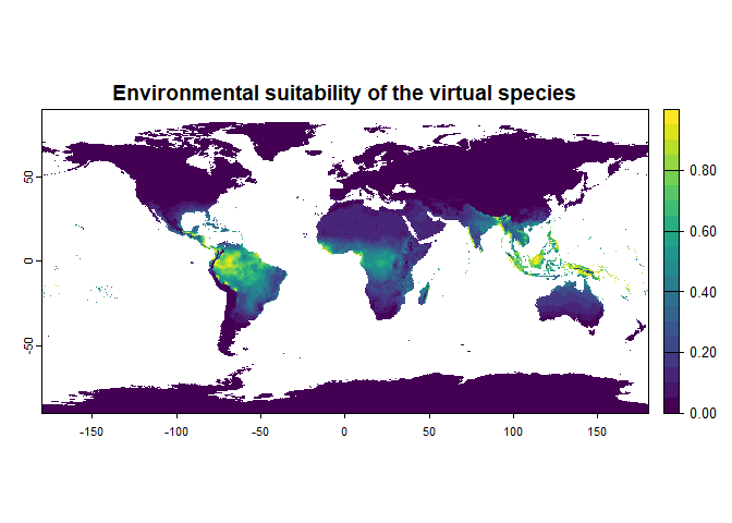
my.first.species## Virtual species generated from 2 variables:
## bio1, bio12
##
## - Approach used: Responses to each variable
## - Response functions:
## .bio1 [min=-54.72435; max=30.98764] : dnorm (mean=25; sd=5)
## .bio12 [min=0; max=11191] : dnorm (mean=4000; sd=2000)
## - Each response function was rescaled between 0 and 1
## - Environmental suitability formula = bio1 * bio12
## - Environmental suitability was rescaled between 0 and 1Congratulations! You have just generated your first virtual species distribution, with the default settings. In the next section you will learn about the simple, yet important settings of this function.
2.2. Customisation of parameters
The function generateSpFromFun proceeds into four
important steps:
- The response to each environmental variable is calculated according to the user-chosen functions.
- Each response is rescaled between 0 and 1. This step can be disabled.
- The responses are combined together to compute the environmental suitability. The user can choose how to combine the responses.
- The environmental suitability is rescaled between 0 and 1. This step can be disabled.
2.2.1. Response functions
You can use any existing function with
generateSpFromFun, as long as you provide the necessary
parameters. For example, you can use the function dnorm
shown above, if you provide the parameters mean and
sd:
formatFunctions(bio1 = c(fun = 'dnorm', mean = 25, sd = 5)).
Naturally you can change the values of mean and
sd to your needs.
You can also use the basic functions provided with the package:
- Linear function:
formatFunctions(bio1 = c(fun = 'linearFun', a = 1, b = 0))\[ f(bio1) = a * bio1 + b \]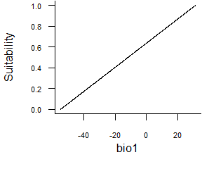
Fig. 2.3 Linear response function
- Quadratic function:
formatFunctions(bio1 = c(fun = 'quadraticFun', a = -1, b = 2, c = 0))\[ f(bio1) = a \times bio1^2 + b \times bio1 + c\]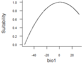
Fig. 2.4 Quadratic response function
- Logistic function:
formatFunctions(bio1 = c(fun = 'logisticFun', beta = 150, alpha = -5))\[ f(bio1) = \frac{1}{1 + e^{\frac{bio1 - \beta}{\alpha}}} \]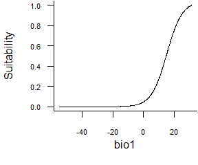
Fig. 2.5 Logistic response function
- Normal function defined by extremes:
formatFunctions(bio1 = c(fun = 'custnorm', mean = 25, diff = 5, prob = 0.99))This function allows you to set extremum of a normal curve. In the example above, we define a response where the optimum is 25°C (mean = 25), and 99% of the area under the curve (prob = 0.99) will be comprised between 20 and 30°C (diff = 50).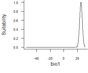
Fig. 2.6 Normal function defined by extremes
- Beta response function (Oksanen & Minchin, 2002, Ecological
Modelling 157:119-129):
formatFunctions(bio1 = c(fun = 'betaFun', p1 = 0, p2 = 25, alpha = 0.9, gamma = 0.08))\[ f(bio1) = (bio1 - p1)^{\alpha} * (p2 - bio1)^{\gamma} \]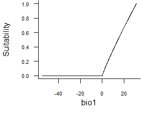
Fig. 2.7 Beta response function
- Or you can create your own functions (see the section How to create your own response functions if you need help for this).
2.2.2. Rescaling of individual response functions
This rescaling is performed because if you use very different
response function for different variables, (e.g., a Gaussian
distribution function with a linear function), then the responses may be
disproportionate among variables. By default this rescaling is enabled
(rescale.each.response = TRUE), but it can be disabled
(rescale.each.response = FALSE).
2.2.3. Combining response functions
There are three main possibilities to combine response functions to
calculate the environmental suitability, as defined by the parameters
species.type and formula:
species.type = "additive": the response functions are added.species.type = "multiplicative": the response functions are multiplied. This is the default behaviour of the function.formula = "bio1 + 2 * bio2 + bio3": if you choose a formula, then the response functions are combined according to your formula (parameterspecies.typeis then ignored).
For example, if you want to generate a species with the same partial
responses as in 2.1, but with a strong importance for temperature, then
you can specify the formula :
formula = "2 * bio1 + bio12"
library(virtualspecies)

my.parameters <- formatFunctions(bio1 = c(fun = 'dnorm', mean = 25, sd = 5),
                                 bio12 = c(fun = 'dnorm', mean = 4000, sd = 2000))

# Generation of the virtual species
new.species <- generateSpFromFun(raster.stack = worldclim[[c("bio1", "bio12")]],
                                 parameters = my.parameters,
                                 formula = "2 * bio1 + bio12",
                                 plot = TRUE)
## Generating virtual species environmental suitability...## - The response to each variable was rescaled between 0 and 1. To
## disable, set argument rescale.each.response = FALSE## - The final environmental suitability was rescaled between 0 and 1. To disable, set argument rescale = FALSE## [1] "2 * bio1 + bio12"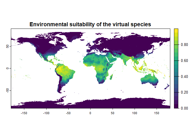
new.species## Virtual species generated from 2 variables:
## bio1, bio12
##
## - Approach used: Responses to each variable
## - Response functions:
## .bio1 [min=-54.72435; max=30.98764] : dnorm (mean=25; sd=5)
## .bio12 [min=0; max=11191] : dnorm (mean=4000; sd=2000)
## - Each response function was rescaled between 0 and 1
## - Environmental suitability formula = 2 * bio1 + bio12
## - Environmental suitability was rescaled between 0 and 1One can even make complex interactions between partial responses:
library(virtualspecies)

my.parameters <- formatFunctions(bio1 = c(fun = 'dnorm', mean = 25, sd = 5),
                                 bio12 = c(fun = 'dnorm', mean = 4000, sd = 2000))

# Generation of the virtual species
new.species <- generateSpFromFun(raster.stack = worldclim[[c("bio1", "bio12")]],
                                 parameters = my.parameters,
                                 formula = "3.1 * bio1^2 - 1.4 * sqrt(bio12) * bio1",
                                 plot = TRUE)
## Generating virtual species environmental suitability...## - The response to each variable was rescaled between 0 and 1. To
## disable, set argument rescale.each.response = FALSE## - The final environmental suitability was rescaled between 0 and 1. To disable, set argument rescale = FALSE## [1] "3.1 * bio1^2 - 1.4 * sqrt(bio12) * bio1"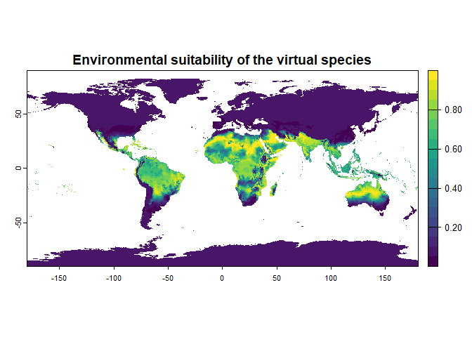
new.species## Virtual species generated from 2 variables:
## bio1, bio12
##
## - Approach used: Responses to each variable
## - Response functions:
## .bio1 [min=-54.72435; max=30.98764] : dnorm (mean=25; sd=5)
## .bio12 [min=0; max=11191] : dnorm (mean=4000; sd=2000)
## - Each response function was rescaled between 0 and 1
## - Environmental suitability formula = 3.1 * bio1^2 - 1.4 * sqrt(bio12) * bio1
## - Environmental suitability was rescaled between 0 and 1Note that this is an example to show the possibilities of the function; I have no idea of the relevance of such a relationship!
2.2.4. Rescaling of the final environmental suitability
This final rescaling is performed because the combination of the
different responses can lead to very different range of values. It is
therefore necessary to allow environmental suitabilities to be
comparable among virtual species, and should not be disabled unless you
have very precise reasons to do it. The argument rescale
controls this rescaling (TRUE by default).
2.3. How to create and use your own response functions
An important aspect of generateSpFromFun is that you can
create and use your own response functions. In this section we will see
how we can do that in practice.
We will take the example of a simple linear function: \[ f(x, a, b) = ax + b\]
Our first step will be to create the function in R:
linear.function <- function(x, a, b)
{
  a*x + b
}
That’s it! You created a function called linear.function
in R.
Let’s try it now:
linear.function(x = 0.5, a = 2, b = 1)## [1] 2linear.function(x = 3, a = 4, b = 1)## [1] 13linear.function(x = -20, a = 2, b = 0)## [1] -40It seems to work properly. Now we will use
linear.function to generate a virtual species distribution.
We want a species responding linearly to the annual mean temperature,
and with a gaussian to the annual precipitations:
my.responses <- formatFunctions(bio1 = c(fun = "linear.function", a = 1, b = 0),
                                bio12 = c(fun = "dnorm", mean = 1000, sd = 1000))

generateSpFromFun(raster.stack = worldclim[[c("bio1", "bio12")]],
                  parameters = my.responses, plot = TRUE)
## Generating virtual species environmental suitability...## - The response to each variable was rescaled between 0 and 1. To
## disable, set argument rescale.each.response = FALSE## - The final environmental suitability was rescaled between 0 and 1. To disable, set argument rescale = FALSE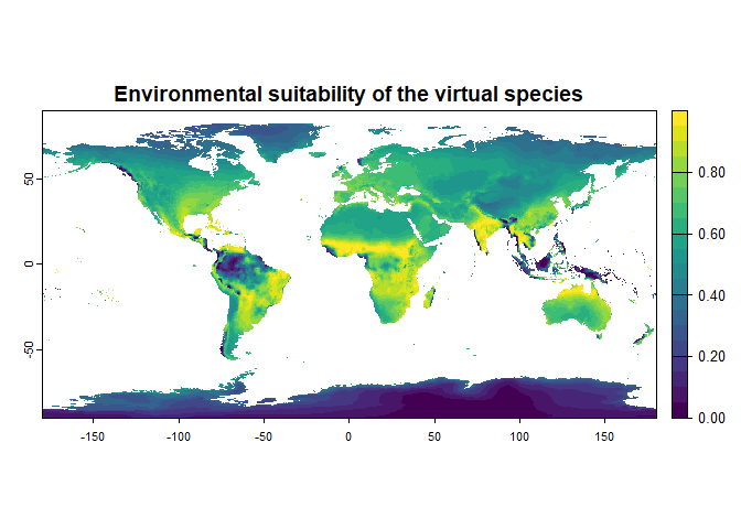
## Virtual species generated from 2 variables:
##  bio1, bio12
##
## - Approach used: Responses to each variable
## - Response functions:
##    .bio1  [min=-54.72435; max=30.98764] : linear.function   (a=1; b=0)
##    .bio12  [min=0; max=11191] : dnorm   (mean=1000; sd=1000)
## - Each response function was rescaled between 0 and 1
## - Environmental suitability formula = bio1 * bio12
## - Environmental suitability was rescaled between 0 and 1
And it worked! Your turn now!
-----------------
Do not hesitate if you have a question, find a bug, or would like to add a feature in virtualspecies: mail me!