1. Input data
virtualspecies uses spatialised environmental data as an
input. These data must be gridded spatial data in the
SpatRaster format of the package terra.
1.1. Small introduction to raster data
The input data for virtual species is gridded spatial data
(i.e., raster data).
To summarise, a raster is a map regularly divided into small units,
called pixels. Each pixel has its own value. These values can be, for
example, temperature values, for a raster of temperature. Raster data
can be imported into R using the package terra. The command
rast() will allow you to import your own rasters (stored on
your hard drive) into an object of class SpatRaster. Below
you will find some concrete examples.
1.2. Required format for virtualspecies
As stated above, the required format is a SpatRaster
containing all the environmental variables with which you want to
generate a virtual species distribution. Note that I may use
interchangeably the terms ‘variables’ and ‘layers’ in this tutorial,
because they roughly refer to the same aspect: a layer is the spatial
representation of an environmental variable.
The most important part here is that every layer of your
SpatRaster must be correctly named, because these names
will be used when generating virtual species.
Hence, I strongly advise using explicit names for your layers. You can
use “variable1”, “variable2”, etc. or “layer1”, “layer2”, etc. but names
like “bio1”, “bio2”, “bio3”, (bioclimatic variable names) or
“temp1”, “temp2”, etc. will reduce confusion.
You can access the names of the layers of your stack with
names(my.stack), and modify them with
names(my.stack) <- c("name1", "name2", etc.).
1.3. A quick and easy example using WorldClim data
WorldClim (www.worldclim.org) freely provides gridded climate data
(temperature and precipitations) for the entire World. These data can be
downloaded to your hard drive from the website above, and then imported
into R using the stack command:
rast("my_path/worldclim_data.tif").
Otherwise, a much simpler solution is to directly download them into
R using the R package geodata, with the function
worldclim_global() (requires an internet connection).
You have to provide the type of environmental variables you are looking for:
- tavg = average monthly mean temperature (°C * 10)
- tmin = average monthly minimum temperature (°C * 10)
- tmax = average monthly maximum temperature (°C * 10)
- prec = average monthly precipitation (mm)
- srad = incident solar radiation (kJ m-2 day-1)
- wind = wind speed (2m above the ground) (m.s-1)
- bio = bioclimatic variables derived from the tmean, tmin, tmax and prec
- vapr = vapor pressure (kPa)
And the resolution: 0.5, 2.5, 5, or 10 minutes of a degree. Note that at fine resolutions the files downloaded are very heavy and may take a long time.
You need to specify the directory where the files will be downloaded.
Below, I used a temporary directory created by R
(path = tempdir()), but this is not an optimal choice,
since we will probably have to redownload everytime. You should probably
create a dedicated folder and specify it in path, e.g.
path = "gis_data".
Here is the example in practice:
library(geodata)
worldclim <- worldclim_global(var = "bio", res = 10,
                              path = tempdir())
worldclim
## class : SpatRaster
## dimensions : 1080, 2160, 19 (nrow, ncol, nlyr)
## resolution : 0.1666667, 0.1666667 (x, y)
## extent : -180, 180, -90, 90 (xmin, xmax, ymin, ymax)
## coord. ref. : lon/lat WGS 84 (EPSG:4326)
## sources : wc2.1_10m_bio_1.tif
## wc2.1_10m_bio_2.tif
## wc2.1_10m_bio_3.tif
## ... and 16 more source(s)
## names : wc2.1~bio_1, wc2.1~bio_2, wc2.1~bio_3, wc2.1~bio_4, wc2.1~bio_5, wc2.1~bio_6, ...
## min values : -54.72435, 1.00000, 9.131122, 0.000, -29.68600, -72.50025, ...
## max values : 30.98764, 21.14754, 100.000000, 2363.846, 48.08275, 26.30000, ...You can see that the object is of class SpatRaster,
ready to use for virtualspecies. The names of the layers
are also convenient.
We can easily access a subset of the layers with
[[]]:
# The first four layers
worldclim[[1:4]]
## class : SpatRaster
## dimensions : 1080, 2160, 4 (nrow, ncol, nlyr)
## resolution : 0.1666667, 0.1666667 (x, y)
## extent : -180, 180, -90, 90 (xmin, xmax, ymin, ymax)
## coord. ref. : lon/lat WGS 84 (EPSG:4326)
## sources : wc2.1_10m_bio_1.tif
## wc2.1_10m_bio_2.tif
## wc2.1_10m_bio_3.tif
## wc2.1_10m_bio_4.tif
## names : wc2.1_10m_bio_1, wc2.1_10m_bio_2, wc2.1_10m_bio_3, wc2.1_10m_bio_4
## min values : -54.72435, 1.00000, 9.131122, 0.000
## max values : 30.98764, 21.14754, 100.000000, 2363.846# Layers bio1 and bio12 (annual mean temperature and annual precipitation)
worldclim[[c("wc2.1_10m_bio_1", "wc2.1_10m_bio_12")]]## class : SpatRaster
## dimensions : 1080, 2160, 2 (nrow, ncol, nlyr)
## resolution : 0.1666667, 0.1666667 (x, y)
## extent : -180, 180, -90, 90 (xmin, xmax, ymin, ymax)
## coord. ref. : lon/lat WGS 84 (EPSG:4326)
## sources : wc2.1_10m_bio_1.tif
## wc2.1_10m_bio_12.tif
## names : wc2.1_10m_bio_1, wc2.1_10m_bio_12
## min values : -54.72435, 0
## max values : 30.98764, 11191And we can plot our variables:
# Plotting bio1 and bio12
plot(worldclim[[c("wc2.1_10m_bio_1", "wc2.1_10m_bio_12")]])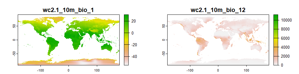
-----------------
Do not hesitate if you have a question, find a bug, or would like to add a feature in virtualspecies: mail me!